精读|从词袋分类器到 Jev:决策模型的发展脉络

原文全文摘录 + 中文翻译 + 精读批注
- 原文:Language Models for Text Classification: From Bag-of-Words to Jev
- 作者:Sebastian Raschka
- 发布:2026-09-29
- 阅读方式:按原文顺序,全文摘录英文原文,每节之后附中文翻译与批注;配图沿用原文插图。
- 版权归原作者所有。本文的翻译与批注由我撰写,与原作者无关。
引言:Jev 到底是什么
The recently released Jev AI model has been quite a cultural phenomenon in technical communities in the past 2 weeks.
While Jev aims to classify things, it’s easy to dismiss Jev as “just a classifier,” and my own view of Jev has evolved quite a bit over the past few days. In particular, my thoughts went from “classifiers used to be my bread & butter; I can easily build this myself” (more on this later) to “wow, this actually works better than I thought.”
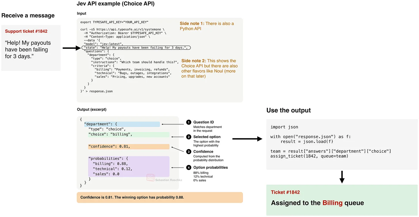
Figure 1: Quick overview of the Jev API; more details on that later.
Sure, the latest state-of-the-art GPT and open-weight LLMs can do the same kinds of classification tasks as Jev, while also being capable of much more general decision-making. But Jev’s advantage is that it can handle those classification tasks much faster and more cheaply.
At the other end of the spectrum, for a narrow, well-defined problem, Jev probably won’t classify anything better, faster, or cheaper than a special-purpose classifier. But its selling point is that it is far more general than those task-specific models.
So, what is the methodology behind Jev (based on an educated guess), what can it do, and why is it so popular? I aim to answer all of these later in this article. However, I thought starting with a brief history of language models for decision-making would be a great way to begin. And it hopefully helps demystify some of the hype and show what Jev does very well (“Jev is essentially a text classifier,” but “Jev is also not ‘just’ a text classifier.”)
PS: I am not affiliated with Jev in any way. Also, I am not offered free access to Jev, and this is also not a product endorsement, just a technical article to offer some insights into the history of text classification to help you make sense of the recent hype.
Since this is a long article, I recommend reading it in your browser, where you can access the table of contents menu on the left side.
最近发布的 Jev AI 模型在过去两周里成了技术社区的一种文化现象。
虽然 Jev 的目标是做分类,但很容易把它轻视为“只是一个分类器”。我自己对 Jev 的看法在过去几天里也演变了不少:从“分类器曾是我的看家本领,我自己随手就能造一个”(后面细说),变成了“哇,实际效果比我想的好”。
图 1:Jev API 速览,细节后文展开。
当然,最新的 SOTA GPT 和开源 LLM 也能做 Jev 能做的同类分类任务,还能做更通用的决策。但 Jev 的优势在于:处理这些分类任务更快、更便宜。
在光谱的另一端,对于窄而明确的问题,Jev 大概不会比专用分类器分得更好、更快、更便宜。但它的卖点是比那些任务专用模型通用得多。
那么,Jev 背后的方法论是什么(基于有根据的推测)?它能做什么?为什么这么火?本文后面会逐一回答。不过我觉得,先简要回顾一下用于决策的语言模型史,是个很好的开场,也希望能祛魅一些炒作,讲清楚 Jev 真正擅长什么(“Jev 本质上是一个文本分类器”,但“Jev 也不‘只’是一个文本分类器”)。
附:我与 Jev 没有任何关联,也没拿免费额度,这不是产品背书,只是一篇技术文章,希望用文本分类的历史帮你理解最近的热潮。
文章很长,**建议在浏览器里读原文**,左侧有目录菜单。
【批注】 开头 “bread & butter → wow” 的转折是全文可信度的地基:作者不是外行惊叹,而是亲手能造分类器的人被说服了,他说好才值钱。另补两个细节:一是 TypeSafe 官博标题里的 “System One” 借的是 Kahneman 快/慢思考——System 1 快、直觉、便宜,Jev 的定位就是决策层的 System 1,名字本身就是产品宣言;二是注意时间锚点,Jev 发布才两周,GPT-6、Opus 5.5 都是 2026 年的代号,读的时候别拿旧年份的经验套。
1. 前 Transformer 时代的语言建模与分类
For completeness, before we put Jev in context (no pun intended), I thought it made the most sense to start chronologically. In this section, I want to take a brief tour of applied text classification via naive Bayes, logistic regression, and the more classic (deep) neural networks before transformer-based models came along.
为了完整起见,在把 Jev 放进上下文(不是双关)之前,按时间顺序讲最合理。这一节快速巡览 Transformer 之前的实用文本分类:朴素贝叶斯、逻辑回归,以及更经典的(深层)神经网络。
1.1 词袋:朴素贝叶斯、逻辑回归和 XGBoost
Back in the day, when I was a grad student 15 years ago, even though recurrent neural networks already existed (more on that later), text classification was usually done with a bag-of-words representation because it was straightforward and could get good results on moderately sized datasets.
In short, we can think of the bag-of-words representation as a method that makes free-form text input of different lengths compatible with classic classifiers (naive Bayes, Logistic Regression, SVMs, Random Forest, XGBoost, to name a few), which expect a fixed-size input vector.
Popular real-world applications include anything from news article classification to email spam filtering. And yes, allegedly even Gmail’s original spam filter used a Naive Bayes model with a bag-of-words representation.
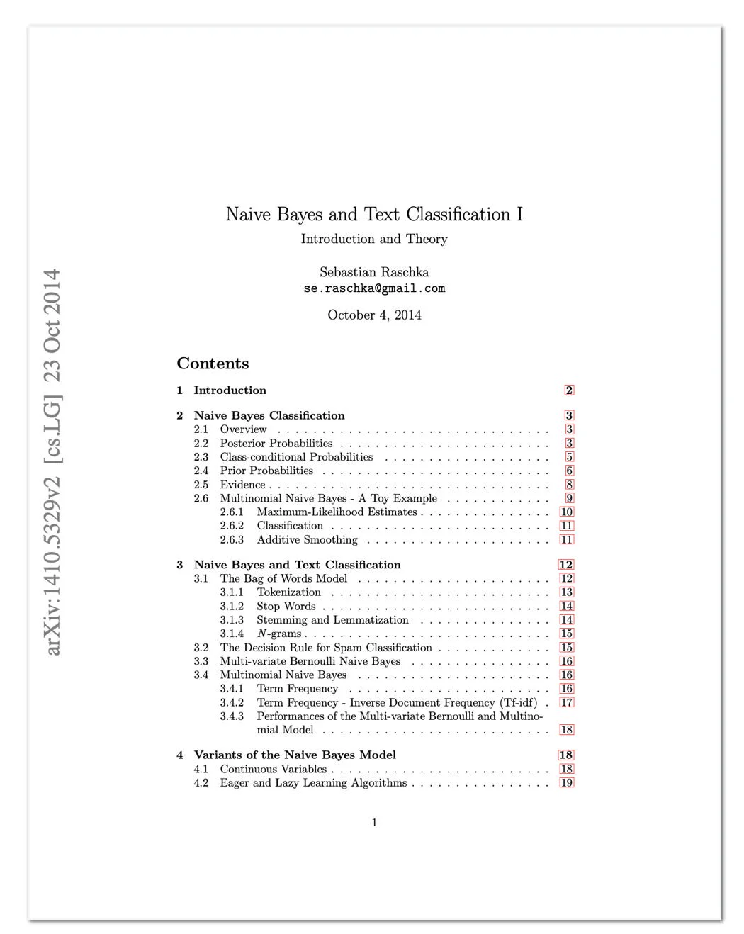
As a side note, I wrote about this approach exactly 12 years ago. It was one of the first things I shared on arXiv.
Figure 2: An old tutorial of mine from 2014 that explains naive Bayes classifiers using a bag-of-words model.
(Text classification with Naive Bayes goes back to at least 1961, where it was used to sort computer abstracts; see the Automatic Indexing: And Experimental Inquiry paper.)
So, what exactly is this bag-of-words representation? It’s a way to convert free-form texts with different lengths, e.g.,
- Training example 1: “Zentropa is the most original movie I’ve seen in years. If you like unique thrillers that are influenced by film noir, then this is just the right cure for all of those Hollywood summer blockbusters clogging the theaters these days. Von Trier’s follow-ups like Breaking the Waves have gotten more acclaim, but this is really his best work.”
- Training example 2: “This film is just plain horrible. John Ritter doing pratt falls, 75% of the actors delivering their lines as if they were reading them from cue cards, poor editing, horrible sound mixing”
- Training example 3: “Zentropa has much in common with The Third Man, another noir-like film set among the rubble of postwar Europe.”
into a fixed-size representation for the aforementioned “classic” classifiers. (The example above is an excerpt from the popular IMDb movie review classification dataset.)
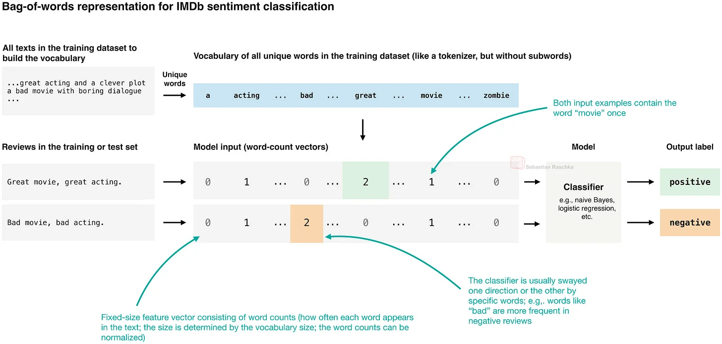
Figure 3: An illustration of a bag-of-words representation.
A bag-of-words model starts by building the vocabulary, which consists of all unique words in the training set (optionally, one can get rid of so-called stopwords like “a” and “the”, which are words that carry little to no semantic meaning in most contexts).
A bag-of-words representation results in these fixed-size inputs by assigning each word in a vocabulary its own position in a vector. We then count how often each word occurs in a document. For example, if we have a vocabulary of 50,000 unique words, it produces a fixed-size vector with 50,000 entries, regardless of whether the input consists of only ten words or 300k words. Note that most entries are zero because each document contains only a small subset of the vocabulary. (Instead of representing the raw counts, there are also normalization schemes like TF-IDF.)
Then, once we have these word frequency vectors, we can train a classifier on a labeled training set, such as emails labeled as spam or non-spam. For example, a logistic regression model would then learn feature weights that correlate certain words (and word counts) with particular labels. For instance, certain words might increase the predicted spam probability, and others may decrease it.
This approach is computationally cheap and can work well when particular words provide strong clues about the label. In a simple classification task such as spam classification, this is often enough to get quick, reasonably accurate results.
But one of the biggest downsides of this approach is that, because of the nature of the bag-of-words representation, it loses word order. So, for example, “the dog bites the man” and “the man bites the dog” produce identical vectors despite describing different events.
(There are some workarounds to preserve some local order by adding word pairs or longer sequences, called n-grams, as features, although this increases the vocabulary size.)
Despite the shortcomings, I still think that a bag-of-words has its place in certain low-stakes applications because it’s so cheap, and a bag-of-words representation + logistic regression remains my go-to baseline for every text classification problem, since it’s so easy to implement.
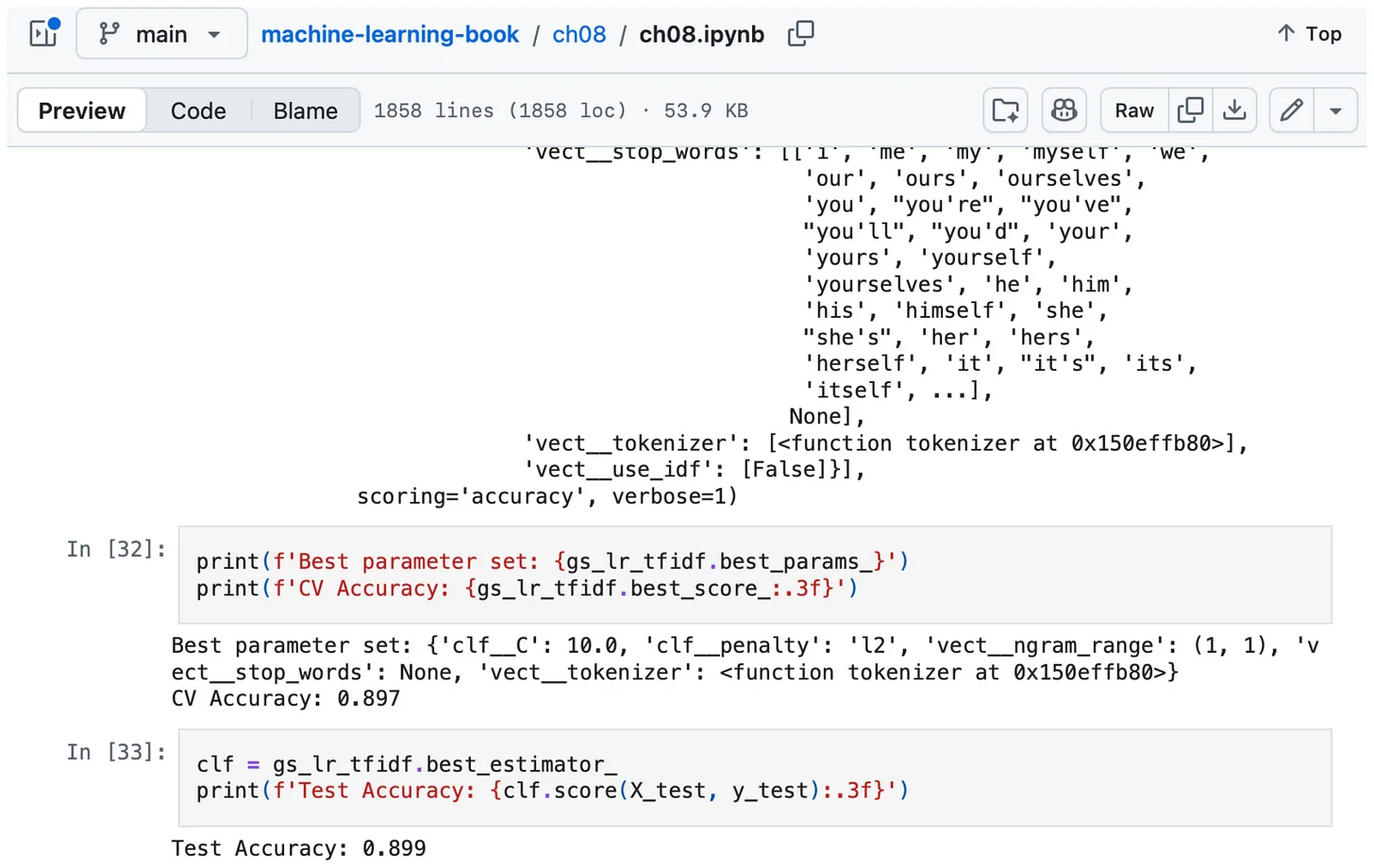
Figure 4: For those interested in building a simple logistic regression classifier, I have a tutorial up here. This model achieves 89.9% accuracy (on a balanced dataset).
想当年,15 年前我读研究生时,虽然循环神经网络已经存在(后文细说),但文本分类通常还是用词袋表示,因为它直接,在中等规模数据集上效果不错。
简单说,词袋表示是一种办法,把长短不一的自由文本输入,变成经典分类器(朴素贝叶斯、逻辑回归、SVM、随机森林、XGBoost 等)能吃的定长输入向量。
流行的实际应用从新闻分类到邮件垃圾过滤都有。对,据说 Gmail 最早的垃圾过滤器就是朴素贝叶斯 + 词袋。
顺带一提,12 年前我写过这个方法,那是我最早发在 arXiv 上的东西之一。
图 2:我 2014 年用词袋讲朴素贝叶斯分类器的旧教程。
(朴素贝叶斯做文本分类至少可以追溯到 1961 年,当时用来给计算机文摘排序,见 Automatic Indexing: And Experimental Inquiry。)
那么词袋表示到底是什么?它把长短不一的自由文本,例如:
- 训练例 1:*”Zentropa 是我多年来见过最有原创性的电影……这是他最好的作品。”*
- 训练例 2:*”这电影简直糟透了……剪辑稀烂,混音糟糕”*
- 训练例 3:*”Zentropa 和《第三人》很像,另一部设在战后欧洲废墟中的黑色电影。”*
变成定长表示,喂给上面说的“经典”分类器。(上例摘自流行的 IMDb 影评分类数据集。)
图 3:词袋表示示意。
词袋模型先建词汇表,即训练集中所有不重复词(可选去掉 “a””the” 这类停用词,它们在多数语境下几乎没有语义)。
词袋表示给词汇表中每个词在向量里分配一个固定位置,然后数每个词在文档里出现几次。比如词汇表有 5 万个词,不管输入是 10 个词还是 30 万词,都产出 5 万维的定长向量。注意多数位置是 0,因为每篇文档只用到词汇表的一小部分。(除了原始计数,也有 TF-IDF 这类归一化方案。)
有了词频向量,就可以在有标注的训练集(比如标了垃圾/非垃圾的邮件)上训练分类器。例如逻辑回归会学到特征权重,把某些词(及词频)和特定标签关联起来:有些词推高垃圾概率,有些词压低它。
这办法计算便宜,当某些词本身就是标签的强线索时效果很好。在垃圾分类这种简单任务上,经常能又快又准。
但它最大的缺点之一是丢失了词序。比如 “the dog bites the man”(狗咬人)和 “the man bites the dog”(人咬狗)会产出完全相同的向量,尽管说的完全是两件事。
(有变通办法:把词对或更长的序列(n-gram)也加进特征,保留一点局部顺序,但代价是词汇表变大。)
尽管有缺点,我仍觉得词袋在某些低风险应用里有一席之地,因为它太便宜了。词袋表示 + 逻辑回归至今仍是我做每个文本分类问题时的首选基线,因为实现太容易了。
图 4:想自己搭个简单的逻辑回归分类器可以看这里。这个模型在(平衡数据集上)达到 89.9% 准确率。
【批注】 补两个原文没展开的词:TF-IDF = 词频 × 逆文档频率,作用是压制”的/是”这类到处都有的词,抬升罕见但区分度高的词;stopwords 之所以叫 stop,是因为早期搜索引擎建索引时遇到它们就”停”(直接跳过)。另注意 “allegedly”——Gmail 用朴素贝叶斯这个说法作者自己都加了”据说”限定,考据党别当实锤。作者花大篇幅讲”过时”方法不是怀旧,是给全篇立标尺:89.9% 这个基线钉在这里,后面每个新东西(RNN、CNN、Transformer、Jev)都要先赢过它,IMDb 那串数字(89.9→85.66→90.07→95.4→92→96.47)就是这条暗线。
1.2 用于文本分类的深层神经网络
The aforementioned bag-of-words model would also work with (simple) deep neural networks, like multilayer perceptrons. But the downside still is that we would lose the sentence structure and word order.
However, more sophisticated neural network architectures avoid the bag-of-words workaround: convolutional neural networks (CNNs) and recurrent neural networks (RNNs), which can take word embeddings as input.
上面说的词袋模型也能接(简单的)深层神经网络,比如多层感知机。但缺点依旧:丢失句子结构和词序。
不过更精巧的神经网络架构绕开了词袋这个变通:卷积神经网络(CNN)和循环神经网络(RNN),它们可以直接吃词向量。
1.2.1 词向量
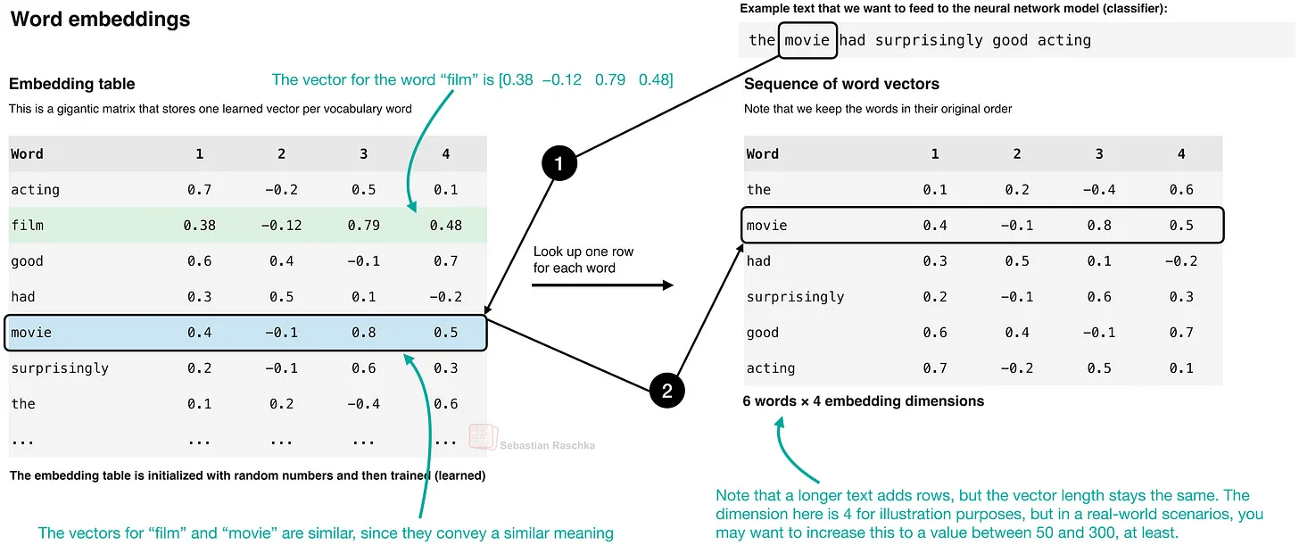
First, before feeding the input texts into a model, we have to convert them into a suitable representation. One such representation is bag-of-words. Another is word embedding vectors. The difference is that a bag-of-words vector represents the entire text by counting how often each vocabulary word occurs, while a word embedding represents an individual word as a dense vector of learned numbers.
Figure 5: Illustration of creating word embeddings.
- Word embeddings work similarly to embedding layers in LLMs, i.e., they convert input tokens into dense vectors. Embeddings can happen outside the model (e.g., two classic, popular methods for learning them are Word2Vec and GloVe), or the embedding layer can be part of the neural network architecture itself and be learned and tuned during model training.
These classic embeddings are context-independent at lookup time. The word “bank”, for example, gets the same vector in “river bank” and “bank account” (as you may know, context can be handled via concepts like attention).
For additional resources on embeddings, you may find the following ones helpful:
- Chapter 2: Working with Text Data (this is an LLM chapter but should give you the gist of embedding words or tokens; in LLM tokenizers, we split words into subword tokens; in Word2Vec, 1 word is usually 1 token.)
- Understanding the Difference Between Embedding Layers and Linear Layers (this is an illustration that shows when embedding vectors are mathematically equivalent to Linear layers and matrix multiplications.)
首先,把输入文本喂进模型之前,得先转成合适的表示。词袋是一种,词向量是另一种。区别在于:词袋向量是对整篇文本数词频,而词向量是给每个词学一个稠密数字向量。
图 5:词向量生成示意。
- 词向量和 LLM 里的 embedding 层原理相似,都是把输入 token 转成稠密向量。Embedding 可以在模型外学好(两个经典流行方法是 Word2Vec 和 GloVe),也可以作为神经网络架构的一部分,在训练中一起学、一起调。
这些经典 embedding 在查表时是上下文无关的:比如 “bank” 在 “river bank”(河岸)和 “bank account”(银行账户)里拿到的是同一个向量(上下文问题可以用 attention 之类的概念处理)。
想深入 embedding 可以看:
- 第 2 章:处理文本数据(这是 LLM 章节,但能帮你理解词/token 的 embedding;LLM 分词器把词切成 subword token,而 Word2Vec 里通常 1 个词就是 1 个 token。)
- 理解 Embedding 层和 Linear 层的区别(用图说明 embedding 向量什么时候在数学上等价于 Linear 层和矩阵乘法。)
1.2.2 循环神经网络(RNN)
Since many of you are probably familiar with recurrent neural networks (RNNs), I will keep this section short. RNNs are a classic go-to neural network architecture for natural language processing, and popular variants go back to the 1980s and early 1990s. Transformers, which were introduced in 2017 (and using the attention mechanisms that were first introduced in RNNs; see my Understanding Large Language Models for a brief timeline), then gradually replaced them in many NLP applications.
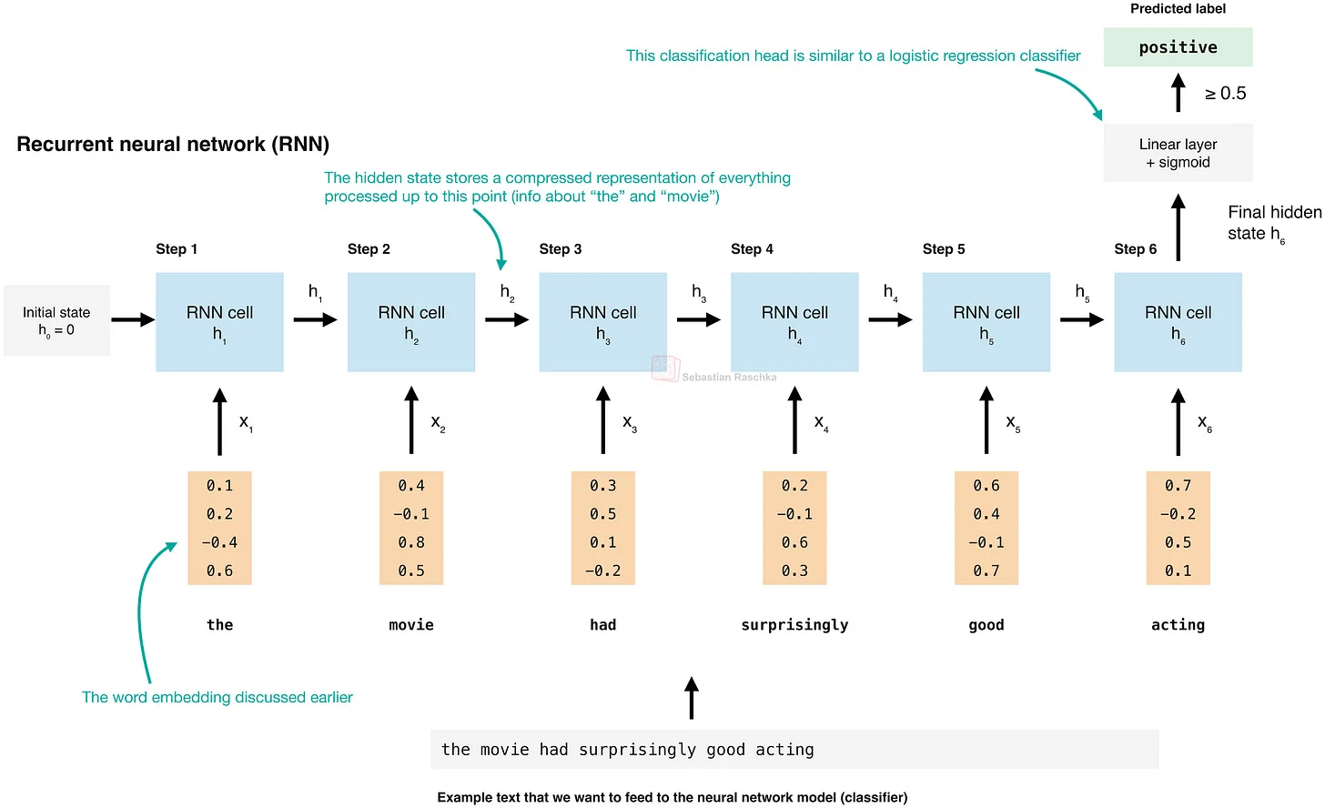
RNNs read a sequence (like text) one word at a time. At each step, they combine the current word embedding (discussed in the previous section) with a hidden state from the previous step. We can think of the hidden state as a fixed-size vector that summarizes the text processed so far, so this makes word order matter, because rearranging the words changes the sequence of state updates.
Figure 6: Illustration of an RNN classifier.
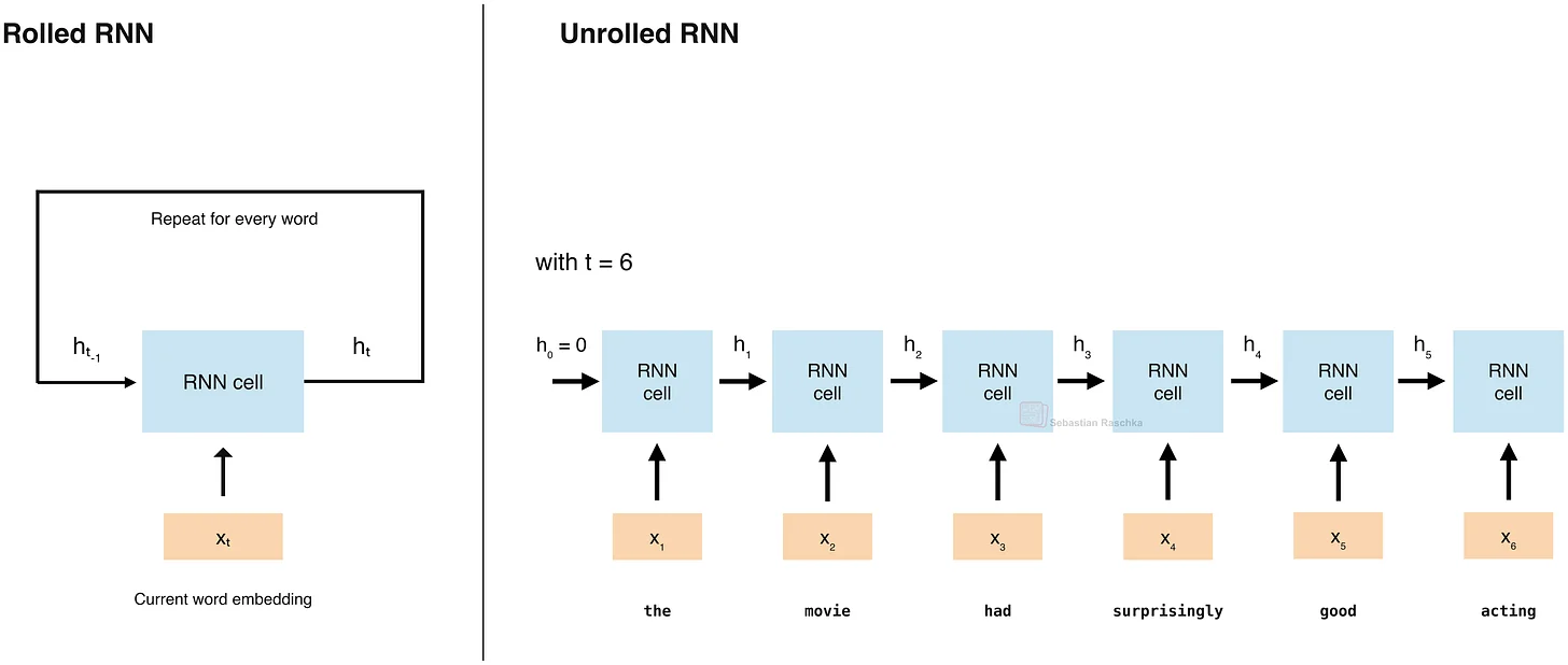
Note that the figure above shows the RNN in the unrolled representation. I.e., the RNN reuses the same layer stack for each input, hence the term “recurrent”. And since it’s “recurrent”, the input text can have an arbitrary length. The figure below illustrates the “recurrence” with the unrolled representation side by side. Note that both show the identical architecture, it’s just a different visualization.
Figure 7: Rolled and unrolled illustration of the same RNN.
RNNs were notoriously hard to train, and there are important improvements to RNNs, like Long short-term memory (LSTM) networks, introduced in 1997, and gated recurrent units (GRUs), introduced in 2014, which use learned gates to control how information is retained and updated. (There is also the more recent xLSTM: Extended long short-term memory, introduced in 2024).
Also, state-space models are inspired by this idea of a fixed-size hidden state updated sequentially, which is cheaper than transformer attention. However, the bottleneck is still how much information the hidden state can retain, and it still has to be processed sequentially. (Fun fact: attention was first developed for RNNs before the transformer architecture came along, but it’s a story for another time; I’ve written about it in my Understanding Large Language Models article.)
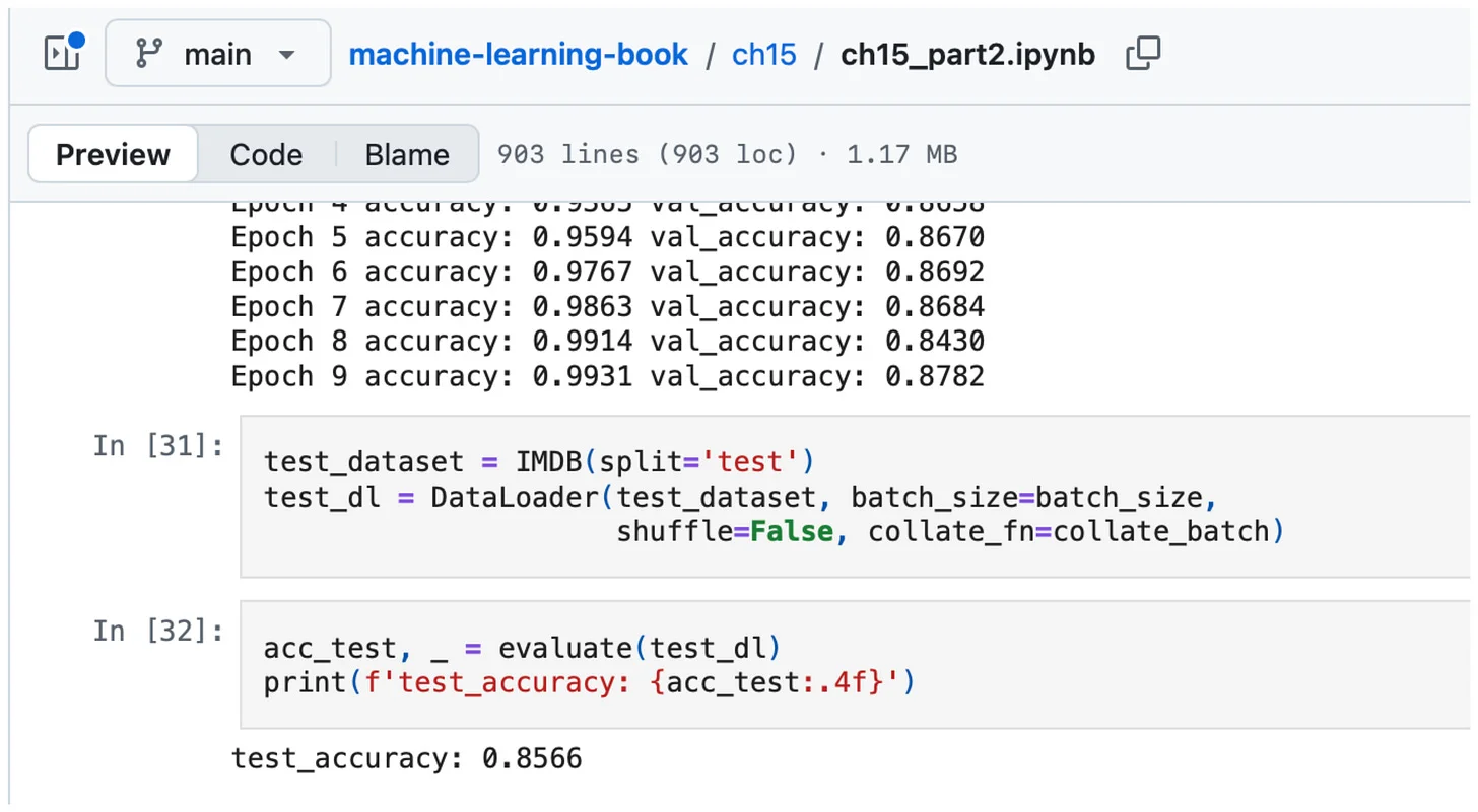
The bottom line is that RNNs can be used to train text classifiers. Coming back to the IMDb movie review dataset, the bag-of-words classifier with logistic regression achieved about 89.9% accuracy (on a balanced dataset), while an LSTM RNN achieved only 85.66% accuracy. Yes, RNNs can be harder to train (stay tuned for the ULMFiT method below, which trains an RNN with much higher accuracy).
Figure 8: A simple RNN with LSTM tutorial. This model achieves 85.66% accuracy (on a balanced dataset); the higher training accuracy indicates substantial overfitting.
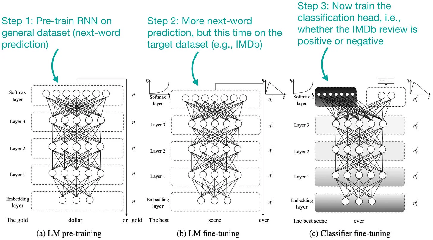
Note that this RNN was trained from scratch. A better approach is to pre-train the model on a larger dataset first, then fine-tune it on this target dataset (classically, we call this approach “transfer learning”).
In the natural language processing domain, one of the most influential papers proposing this approach is ULMFiT (2018), which achieved an impressive 95.4% test accuracy on IMDb.
Figure 9: Annotated figure from the ULMFiT paper.
想必很多人熟悉循环神经网络(RNN),这节从简。RNN 是 NLP 的经典主力架构,流行变体可以追溯到上世纪 80 年代到 90 年代初。2017 年 Transformer 登场(它用的 attention 机制最早其实是在 RNN 里提出来的,时间线见我的 Understanding Large Language Models),之后在很多 NLP 应用里逐步取代了 RNN。
RNN 逐词读序列(比如文本)。每一步把当前词向量(上一节讲的)和上一步的隐状态结合起来。可以把隐状态想成一个定长向量,总结到目前为止读过的内容——这就让词序有了意义,因为打乱词序会改变状态更新的序列。
图 6:RNN 分类器示意。
注意上图画的是 RNN 的展开(unrolled)表示:RNN 对每个输入复用同一组层,所以叫“循环”。正因为“循环”,输入文本可以是任意长度。下图把折叠和展开画法并排放,注意两者是同一个架构,只是可视化不同。
图 7:同一个 RNN 的折叠与展开画法。
RNN 出了名的难训练。重要的改进有 1997 年的长短期记忆(LSTM)和 2014 年的门控循环单元(GRU),用可学习的门控制信息的保留和更新。(还有 2024 年的 xLSTM。)
状态空间模型也受这个思想启发:顺序更新的定长隐状态,比 Transformer attention 便宜。但瓶颈仍在隐状态能记住多少信息,而且必须顺序处理。(冷知识:attention 最早是为 RNN 发明的,早于 Transformer,故事以后讲,我在 Understanding Large Language Models 里写过。)
底线是:RNN 可以用来训练文本分类器。回到 IMDb 影评数据集:词袋 + 逻辑回归约 89.9% 准确率(平衡数据集),而 LSTM RNN 只有 85.66%。是的,RNN 更难训练(下面讲的 ULMFiT 方法能把 RNN 训到高得多,且听下回)。
图 8:带 LSTM 的简单 RNN教程,准确率 85.66%(平衡数据集);训练准确率更高,说明过拟合严重。
注意这个 RNN 是从零训练的。更好的办法是先在大数据集上预训练,再到目标数据集上微调(经典叫法是“迁移学习”)。
NLP 领域提出这个思路最有影响力的论文之一是 ULMFiT(2018),在 IMDb 上达到了惊人的 95.4% 测试准确率。
图 9:ULMFiT 论文的注释版插图。
1.2.3 卷积神经网络(CNN)
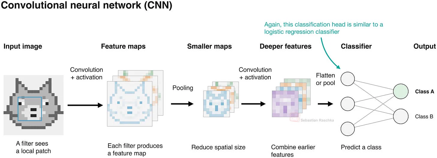
You probably know convolutional neural networks (CNNs) from their use in computer vision. However, it is also possible, although historically less common, to use them for text.
Figure 10: Illustration of a convolutional neural network (CNN) to classify images.
As shown in the image classification example in the figure above, CNNs apply learned filters to image patches (windows). Similarly, in the natural language domain, we can apply learned filters to windows of adjacent word embeddings.
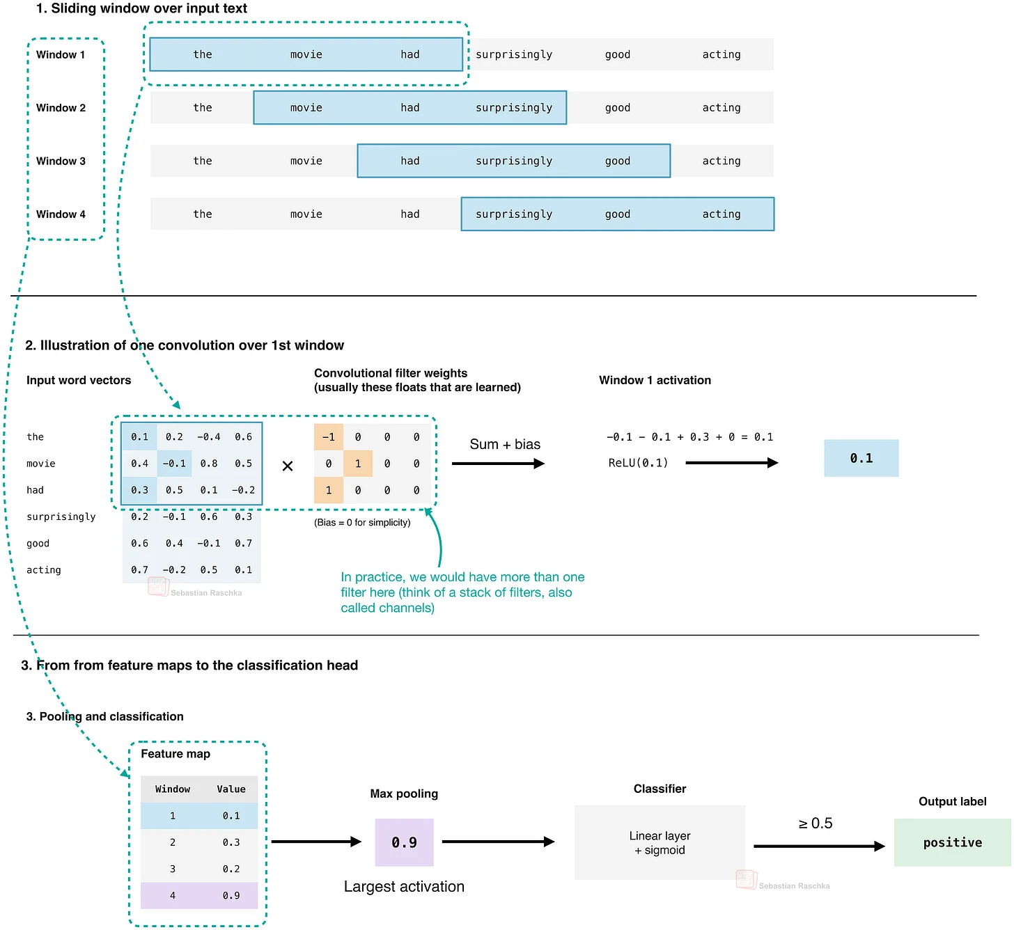
Figure 11: A CNN for text classification, step by step. Only 1 filter (channel) for simplicity.
As illustrated in the figure above, a convolutional filter with a window size of three uses the same weights for each adjacent group of three words. Then, as it slides over the inputs, it moves the filter one word at a time across “the movie had surprisingly good acting”. So, this gives four windows (ignoring padding for simplicity):
- 1: “the movie had”
- 2: “movie had surprisingly”
- 3: “had surprisingly good”
- 4: “surprisingly good acting”
So, in the last layer, before the classification head, we can either flatten or global max pool the results before connecting it to the classification head. While flattening preserves all information, it would produce differently sized vectors depending on the text input length. (E.g., if “the movie had surprisingly good acting” were longer, we would have longer feature maps.) So, to make it input-length agnostic, global max-pooling would be a better option here.
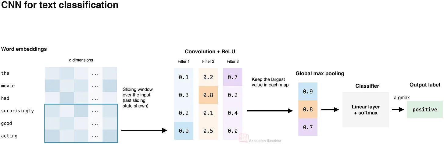
In short, we can visualize the text CNN as shown below.
Figure 12: CNN for text classification with multiple filters (channels).
Also, what’s nice is that the filter computations across positions can run in parallel, which avoids the step-by-step dependency of an RNN.
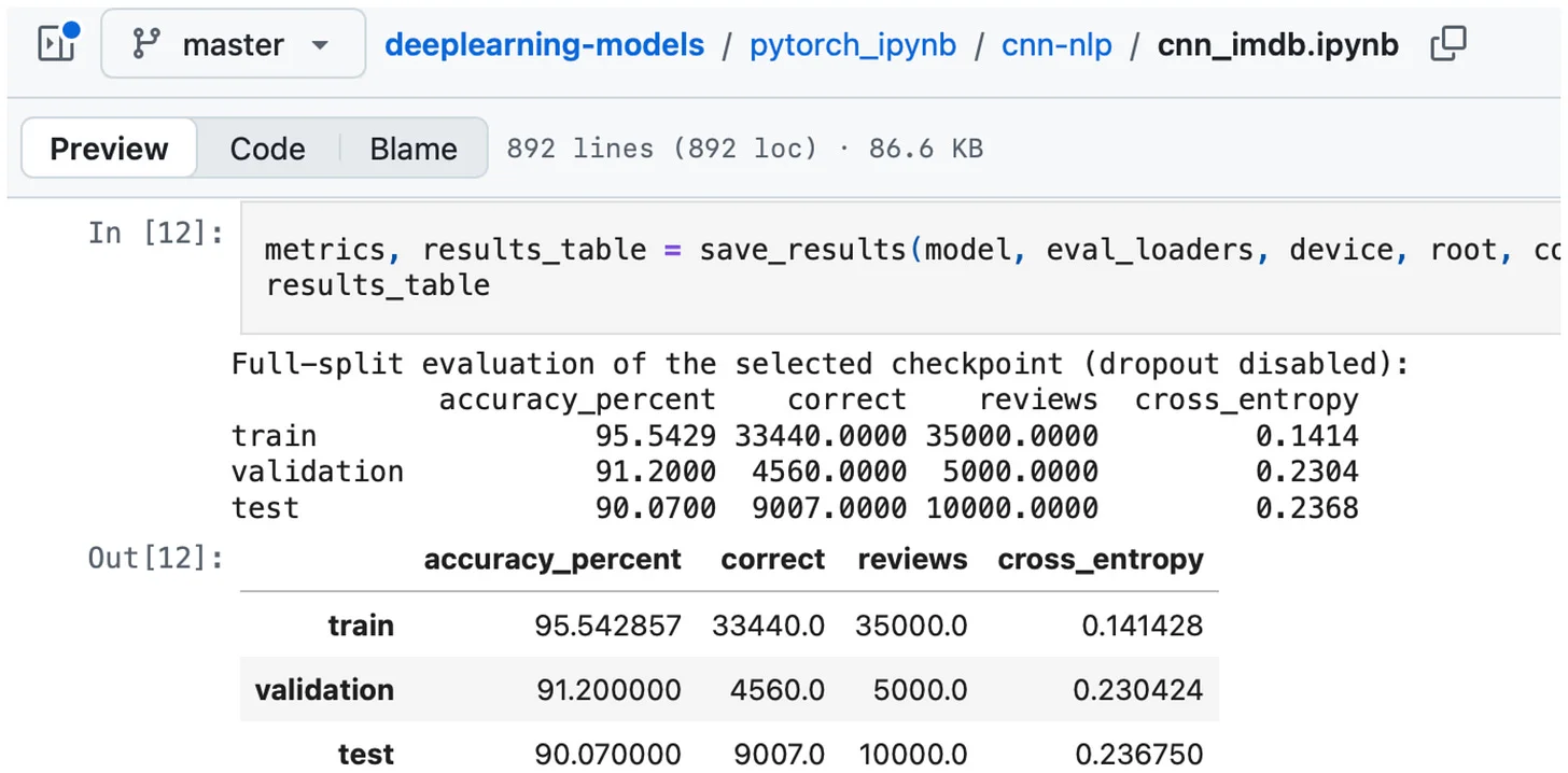
For a quick comparison, on the aforementioned IMDb dataset, my experiments show that such a CNN gets about 90.07% accuracy (but note that this is highly architecture-dependent; for example, you may know from computer vision contexts that accuracies can vary widely). (E.g., the good old AlexNet had a ~62.5% top-1 accuracy on ImageNet, and a ConvNeXt V2-H gets 88.9%.)
Figure 13: A CNN trained to classify IMDb movie reviews; it gets 90.07% accuracy on this balanced dataset. You can find the source code here.
你大概是从计算机视觉里认识卷积神经网络(CNN)的。但它也可以用于文本,只是历史上没那么常见。
图 10:用 CNN 做图像分类示意。
如上图图像分类的例子,CNN 把学到的滤波器作用在图像块(窗口)上。同理,在自然语言里,我们可以把学到的滤波器作用在相邻词向量的窗口上。
图 11:文本 CNN 分步演示,为简单只画 1 个滤波器(通道)。
如上图所示,一个窗口大小为 3 的卷积滤波器,对每组相邻 3 个词用同一套权重。它在输入上滑动,每次移动一个词,扫过 “the movie had surprisingly good acting”,得到 4 个窗口(为简单忽略 padding):
- 1:”the movie had”
- 2:”movie had surprisingly”
- 3:”had surprisingly good”
- 4:”surprisingly good acting”
所以在最后一层、分类头之前,可以把结果展平(flatten)或做全局最大池化(global max pool)再接分类头。展平保留全部信息,但向量长度随输入文本长度变化(比如句子更长,特征图就更长)。所以要做到输入长度无关,全局最大池化是更好的选择。
总之,文本 CNN 可以画成下面这样。
图 12:多滤波器(多通道)的文本 CNN。
还有个好处:不同位置的滤波器计算可以并行,避开了 RNN 的逐步依赖。
快速对比一下:在前面说的 IMDb 数据集上,我的实验显示这种 CNN 约 90.07% 准确率(注意这高度依赖架构;搞过视觉的都知道准确率可以差很多——比如老 AlexNet 在 ImageNet 上 top-1 约 62.5%,而 ConvNeXt V2-H 达到 88.9%)。
图 13:在 IMDb 影评上训练的 CNN,平衡数据集准确率 90.07%,源码在这里。
2. Transformer
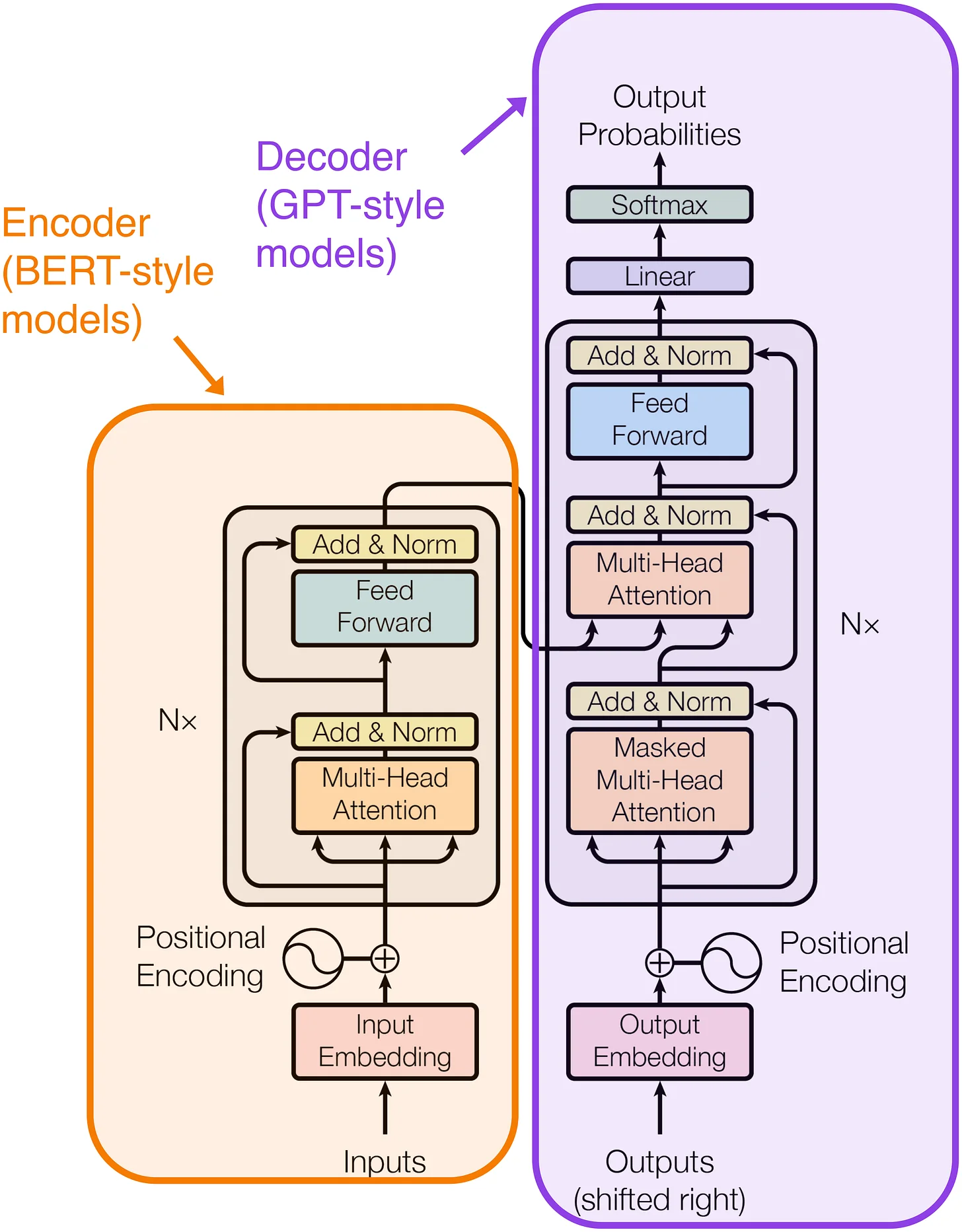
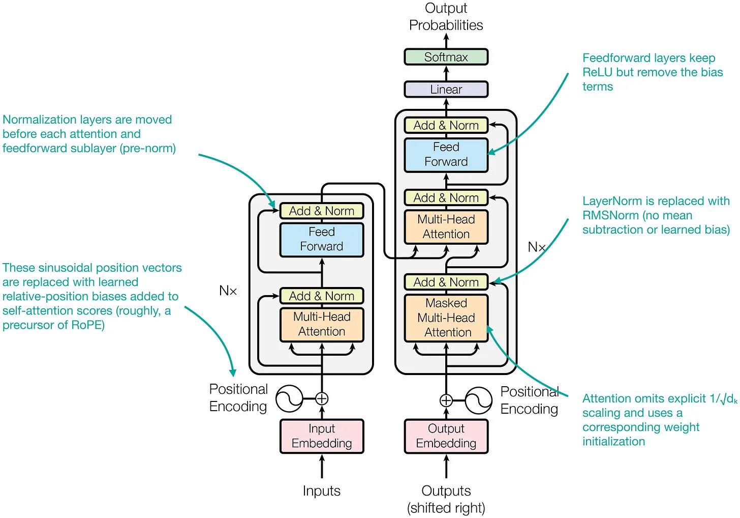
In 2017, the original transformer architecture was introduced in the Attention Is All You Need paper. Since this topic has been covered so extensively (by me and others), I will focus on the classification-relevant aspects. But for those interested in the attention mechanism and other architecture details, please see my related articles on the attention mechanism and architecture comparison (linked in the original article).
The key point is that the original transformer architecture was an encoder-decoder setup used for language translation, but it can be easily adapted for text classification tasks, as I’ll illustrate in the following sections.
Figure 14: The original transformer architecture from Attention Is All You Need.
2017 年,原始 Transformer 架构在 Attention Is All You Need 里登场。这个话题已经被讲烂了(我和别人都讲过),这里只聚焦和分类相关的部分。想看 attention 机制和架构细节的可以去看原文里链的那几篇。
关键点是:原始 Transformer 是为机器翻译设计的 encoder-decoder 结构,但它很容易改造成文本分类任务,后面几节逐一演示。
图 14:Attention Is All You Need 的原始 Transformer 架构。
2.1 Encoder 式语言模型
I remember all too well the first years after the original transformer architecture release. They were pretty much defined by the rivalry between two different approaches:
- Encoder-style models like BERT, primarily developed by Google;
- Decoder-style models like GPT, primarily developed by OpenAI.
Encoder-style models were natural text classifiers, whereas GPT models could do zero- and few-shot classification as an emergent property, but their strength was more in generative tasks.
But let’s start with encoder-style models and how to fine-tune and use them to classify text.
One universal aspect of using transformers, whether encoder- or decoder-style, is that we work with models pre-trained on large text corpora, and, in addition to using them as zero- or few-shot classifiers, we can fine-tune them on the target dataset (similar to ULMFiT, as mentioned in the RNN section earlier).
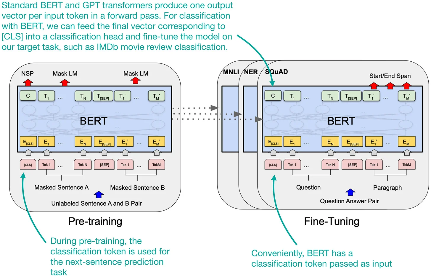
As shown in the figure excerpt from the BERT paper (2018) below, BERT-/encoder-style models have a classification token at the first position that we can conveniently fine-tune for this.
Figure 15: Annotated figure from the original BERT paper.
While BERT models are not nearly as popular as autoregressive GPT-style transformers, thankfully some people still update and modernize them occasionally. One recent example that is often my go-to for classification tasks is the 2024 ModernBERT model.
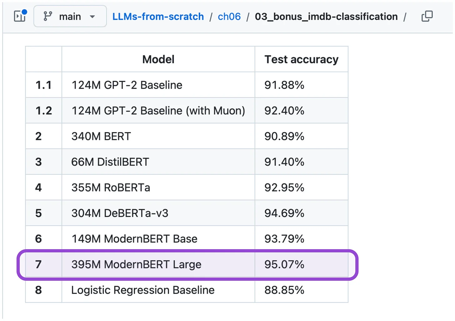
As shown below, on the IMDb movie reviews, ModernBERT gets approximately 95% accuracy with very little fine-tuning effort.
Figure 16: Different LLMs fine-tuned to classify IMDb movie reviews; you can find the source code here. (I did very little hyperparameter tuning, and this can potentially be improved by 1-2% further; however, one of the points here is also that one can get really good results with pretty minimal effort.)
原始 Transformer 发布后的头几年我记得很清楚,基本就是两种路线的 rivalry:
- Encoder 式模型如 BERT,主要是 Google 搞的;
- Decoder 式模型如 GPT,主要是 OpenAI 搞的。
Encoder 式模型天生就是文本分类器,而 GPT 模型是靠涌现能力做零样本/少样本分类,强项还是生成任务。
先从 encoder 式模型讲起:怎么微调、怎么拿来分类。
不管 encoder 还是 decoder,用 Transformer 有个通用套路:在大文本语料上预训练好的模型,除了拿来做零样本/少样本分类,还可以在目标数据集上微调(和前面 RNN 一节讲的 ULMFiT 类似)。
如下图 BERT 论文(2018)的摘录,BERT/encoder 式模型在第一个位置有个分类 token,微调用起来很顺手。
图 15:原始 BERT 论文的注释版插图。
BERT 模型远不如自回归的 GPT 式 Transformer 火,好在还有人时不时更新现代化它们。近期的例子、也是我做分类任务常用的,是 2024 年的 ModernBERT。
如下图,在 IMDb 影评上,ModernBERT 几乎没怎么调就约 95% 准确率。
图 16:微调来分类 IMDb 影评的各种 LLM,源码在这里。(我基本没调超参,还能再涨 1-2 个点;但这里想说的也是:花很小力气就能拿到很好的结果。)
2.2 Decoder 式 LLM
LLMs like GPT are decoder-style, autoregressive transformers that are the center of all attention (no pun intended) for generating text and code.
However, as I explained in chapter 6 of my Build A Large Language Model (From Scratch) book, as a gentle introduction to fine-tuning (before covering instruction fine-tuning), we can also repurpose these for text classification.
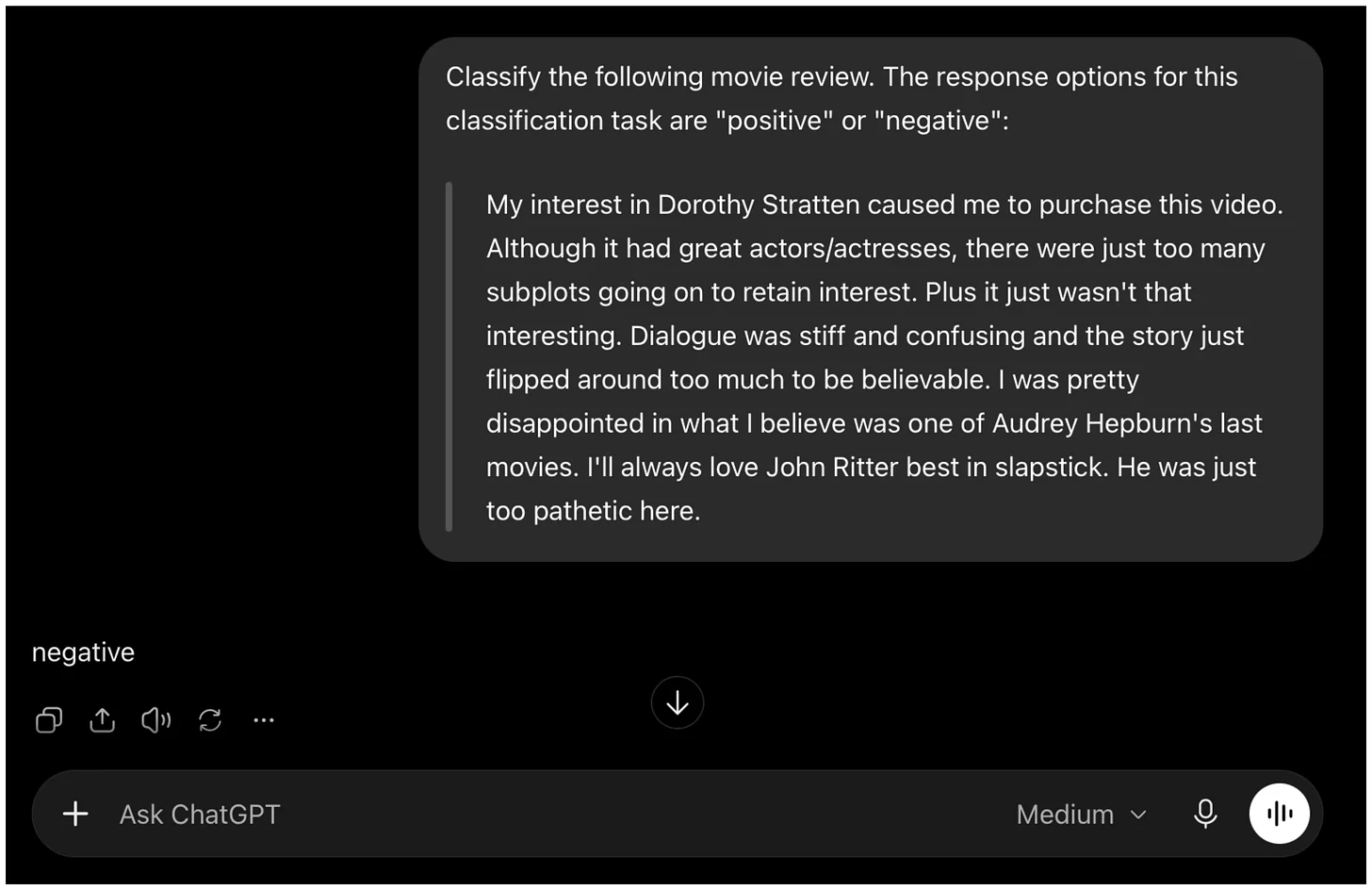
Sure, we can also prompt an LLM directly, as shown in the screenshot below.
Figure 17: Prompting an LLM to classify a movie review.
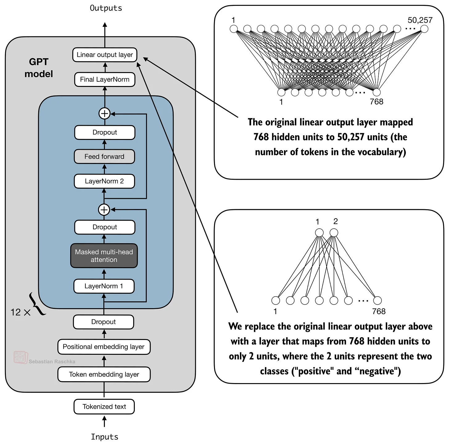
However, if we want structured outputs and we have a specific target domain in mind, this is unnecessarily brittle and inefficient.
Instead, we can replace the output layer with a leaner classification head, as illustrated below:
Figure 18: Swapping the output layer of a GPT-style model with a leaner classification head.
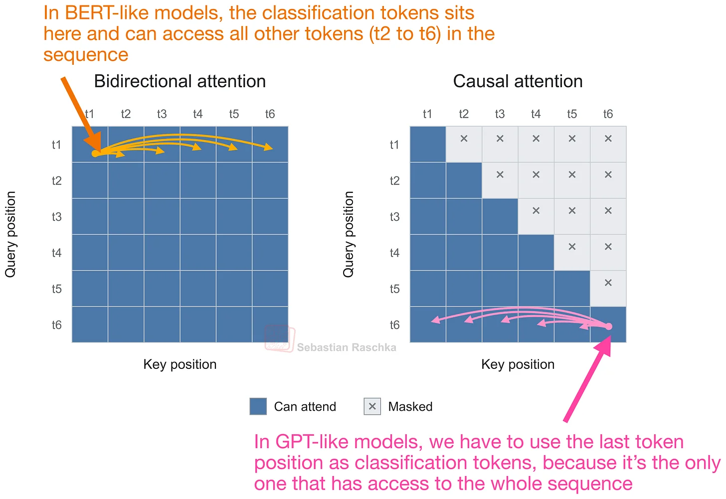
Now, fine-tuning has a few caveats. For instance, because of the autoregressive attention mask, we have to be careful about how we design fine-tuning so that the classification token has information about all other tokens in the sequence.
Figure 19: Attention masks in BERT and GPT.
If you are interested in further technical details, please see my recent end-to-end Building an AI Text Detector From Scratch article.
Overall, though, the advantage of using GPT-style LLMs over e.g., BERT variants is that there are so many modern open-weight architectures out there to adopt. Anything between the small Qwen 3 0.6B models to the latest Kimi, GLM, or DeepSeek models. (Of course, using such >1B parameter models for classification could be a bit overkill from an efficiency perspective, but hey, it’s possible.)
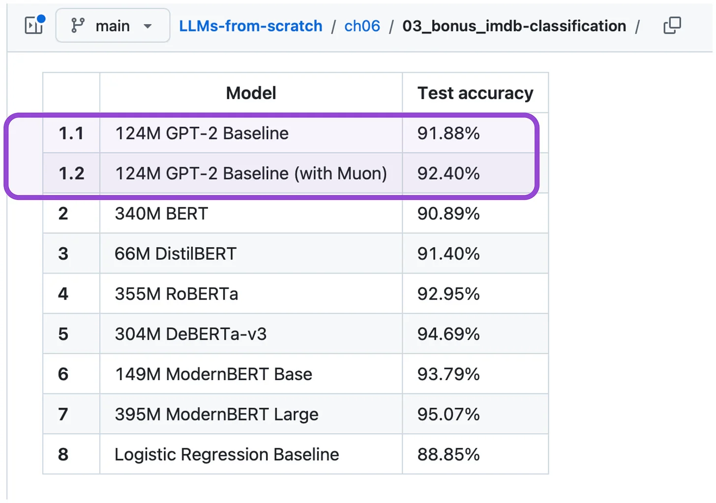
Figure 20: On the aforementioned IMDb movie review dataset, a relatively small GPT-2 124M model gets approximately 92% accuracy; a larger and newer LLM (like a recent Qwen3 variant) would likely perform better.
GPT 这类 LLM 是 decoder 式自回归 Transformer,是生成文本和代码的绝对中心(不是双关)。
但我在 Build A Large Language Model (From Scratch) 第 6 章讲过,作为微调的温和入门(在讲指令微调之前),也可以把它们改造成文本分类器。
当然,也可以直接 prompt LLM,下图是个截图例子。
图 17:prompt LLM 给影评分类。
但如果想要结构化输出、又有明确的目标领域,这么干又脆又浪费。
替代办法是把输出层换成更轻的分类头,如下图:
图 18:把 GPT 式模型的输出层换成轻量分类头。
微调有几个坑。比如因为自回归 attention mask,得小心设计微调,让分类 token 能看到序列里所有其他 token 的信息。
图 19:BERT 和 GPT 的 attention mask。
想看更多技术细节可以看我最近的端到端文章 Building an AI Text Detector From Scratch。
总的来说,用 GPT 式 LLM 而不用 BERT 变体的好处是:外面有太多现代开源架构可以拿来用,从小的 Qwen3 0.6B 到最新的 Kimi、GLM、DeepSeek。(当然,拿 >1B 参数的模型做分类从效率看有点杀鸡用牛刀,但确实可行。)
图 20:在前面说的 IMDb 影评数据集上,相对小的 GPT-2 124M 约 92% 准确率;更大更新的 LLM(比如近期的 Qwen3 变体)大概率更好。
2.3 Encoder-Decoder 式架构
While the original transformer architecture (an encoder-decoder) was split into two paradigms, encoder-style models like BERT and decoder-style LLMs like GPT, there were also efforts to use encoder-decoder-style variants, with the most recent variant (somewhat unexpectedly) being DeepSeek V4.1 Flash. (However, in this case, it’s a causal encoder not a bidirectional one as in T5.)
Keeping the focus on encoder-decoder architectures for classification, probably the most prominent candidate is Google’s 2019 T5 (Text-to-Text Transfer Transformer).
Architecturally, the differences between T5 and the original transformer include updates to the architecture (as summarized below), as well as changes to training. The original transformer was trained to do language translation (in a supervised fashion); T5 uses pre-training on unlabeled text with span corruption, where the encoder receives text with missing spans and the decoder generates those missing spans.
Figure 21: T5 architecture changes to the original transformer architecture. (The architecture drawing is taken from Attention Is All You Need.)
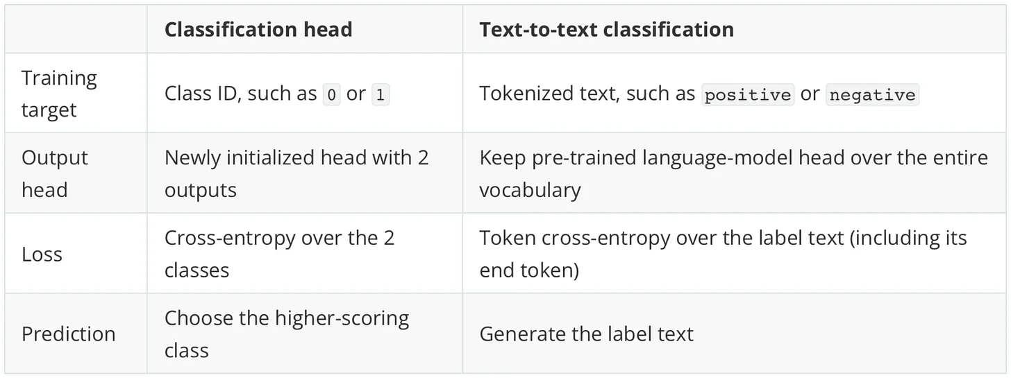
Now, we can use T5 similar to the other RNN, CNN, and transformer approaches above, by adding a classification head.
Additionally, we can also (train to) have the decoder output the class label prediction (like “positive” or “negative” in the IMDb movie review dataset case), similar to regular LLMs. Let’s call this approach text-to-text classification.
While GPT-style LLMs are trained on massive amounts of text, they usually perform text-to-text classification well out of the box, as shown earlier (Figure 17 inserted here again as Figure 22 in the original article for convenience).
Here’s a summary of both approaches for T5:
Figure 23: Classification head vs text-to-text approaches.
For T5, both approaches work, as summarized above. However, in the case of T5, it is common to further fine-tune the decoder to do well on these types of tasks in a given target domain.
原始 Transformer(encoder-decoder)后来分化成 BERT 式 encoder 和 GPT 式 decoder 两条路线,但也有人坚持用 encoder-decoder 变体,最近的例子(有点意外)是 DeepSeek V4.1 Flash。(不过它是 causal encoder,不是 T5 那种双向的。)
聚焦 encoder-decoder 做分类,最知名的候选是 Google 2019 年的 T5 (Text-to-Text Transfer Transformer)。
架构上,T5 相对原始 Transformer 有一些更新(总结如下图),训练方式也变了:原始 Transformer 是有监督训练做机器翻译;T5 在无标注文本上用 span corruption 预训练——encoder 收带缺失片段的文本,decoder 生成这些缺失片段。
图 21:T5 相对原始 Transformer 的架构变化。(架构图取自 Attention Is All You Need。)
T5 可以像上面的 RNN、CNN、Transformer 一样,加个分类头来用。
另外,也可以(训练)让 decoder 直接输出类别标签预测(比如 IMDb 的 “positive”/“negative”),和普通 LLM 一样。这种做法叫 text-to-text 分类。
GPT 式 LLM 在海量文本上训练过,开箱做 text-to-text 分类通常就不错,前面见过(原文为方便把图 17 又贴了一遍作图 22)。
T5 的两种做法总结如下:
图 23:分类头 vs text-to-text 两种做法。
对 T5 两种都行。不过 T5 的常见做法是,在给定目标领域上进一步微调 decoder,让这类任务做得更好。
【批注】 补个词:[CLS] 是 BERT 输入最前面的特殊 token,名字就来自 classification,分类时取它的输出向量,相当于全句的代表。另补个背景:ModernBERT(2024)是 BERT 路线的续命之作(扔掉 NSP、加上 FlashAttention、拉长上下文),说明 encoder 做分类这条线没死,还在进化。作者写 BERT vs GPT rivalry 那段是时代注脚——他亲历了那个 rivalry,点出”分类是 encoder 的主场”,这为后文两处埋线:第 4 章猜 Jev 是”小的 encoder-like 东西”,以及 decoder 也能分类(2.2 节)之所以值得单写一节,正因为它不是主场。
3. Jev 总览
So far, we have seen that there are plenty of approaches to text classification, from traditional methods like logistic regression and naive Bayes with bag-of-words representations to prompting the latest frontier LLMs like GPT-6 or fine-tuning any open-weight LLM with a classification head (or text-to-text classification).
At first, I (almost) dismissed it as “just a classifier,” something that I build routinely for classification tasks with natural language inputs (e.g., see my AI Detector article as a recent public example).
到目前为止我们看到,文本分类的办法多得是:从词袋 + 逻辑回归/朴素贝叶斯这种传统方法,到 prompt 最新的前沿 LLM(如 GPT-6),再到给任意开源 LLM 微调分类头(或 text-to-text 分类)。
起初我(差点)把它当成“只是一个分类器”打发了——这类带自然语言输入的分类任务我平时随手就造(比如最近公开的例子见我的 AI Detector 文章)。
3.1 Jev vs 已有的 text-to-text 分类
Before continuing this discussion, though, let’s start with a quick Jev overview. Jev is a new model released by TypeSafe AI, which just came out of stealth a few weeks ago and got a lot of attention (at first, it seemed a bit bizarre because it looks just like a classifier).
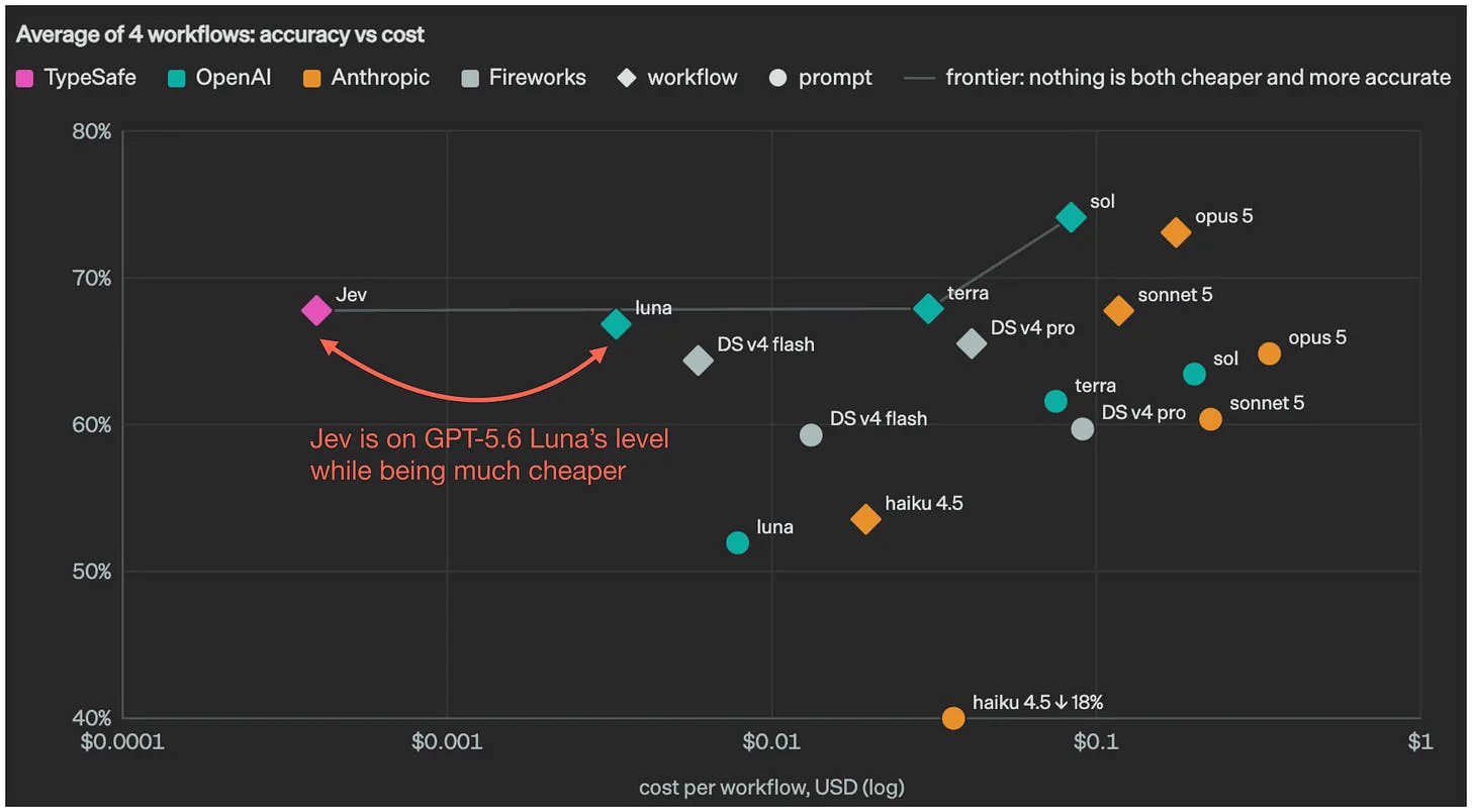
Jev is a proprietary model (although the release was followed by a huge number of quick open-source clones, but we will get to this later) that is relatively cheap to use and claims to be on par with GPT-5.6 Luna (for decision-making) while being orders of magnitude faster and cheaper:
Figure 24: Benchmark from TypeSafe AI blog.
Here, regarding GPT-Luna, think of this as the text-to-text classification approach discussed earlier.
So why all this hype? I think it’s partly because of the nice API and that it performs so well on all kinds of tasks, so it doesn’t require custom fine-tuning.
For example, I can use it to categorize support tickets/emails (I made a video version to show the response time):
Or, I can have the same model play Tetris in real-time (here, I am using the Choice API):
Maybe the best way to succinctly explain it (before getting into technical details) is as follows: Like ChatGPT in 2022 was exciting because it was a general-purpose chat model that could generate all kinds of texts, one of the reasons the tech community is excited about Jev is that it is the ChatGPT moment for classification, where it can cheaply classify all kinds of text inputs without having to fine-tune a custom classifier for each task.
(As of this writing, there’s not much known about the architecture and exact training algorithm, except that one of the founders said it was trained via “Reinforcement Learning for Calibrated Decisions”, but more on that later.)
继续讨论之前,先快速总览 Jev。Jev 是 TypeSafe AI 发布的新模型,几周前刚走出 stealth,引起很大关注(起初有点怪,因为它长得就像个分类器)。
Jev 是闭源模型(发布后跟了一大堆速成的开源克隆,后面讲),用起来相对便宜,宣称决策能力对标 GPT-5.6 Luna,同时快几个数量级、便宜几个数量级:
图 24:TypeSafe AI 博客的 benchmark。
这里的 GPT-Luna,就理解成前面讲的 text-to-text 分类做法。
为什么这么火?我想一方面是 API 好用,另一方面是它在各种任务上表现都很好,不需要逐个微调。
比如,我拿它给客服工单/邮件分类(我还录了视频演示响应速度):
或者,让同一个模型实时玩俄罗斯方块(这里用的是 Choice API):
可能最精炼的解释是(先进技术细节):ChatGPT 在 2022 年让人兴奋,因为它是通用聊天模型,能生成各种文本;技术社区对 Jev 兴奋的理由之一是,它是分类领域的 ChatGPT 时刻——不用给每个任务微调专用分类器,就能便宜地分类各种文本输入。
(写这篇文章时,关于它的架构和确切训练算法所知甚少,只知道一位创始人说它是用“面向校准决策的强化学习”训的,后面细说。)
3.2 Jev 的 API
Over the past few years, we’ve gotten used to throwing bigger, better, and more expensive GPT-style LLMs at all kinds of problems, and for targeted decision-making or classification tasks, a cheap & fast approach like Jev may feel refreshing to most. Especially for one-off tasks where collecting training data and fine-tuning a custom ModernBERT sounds too tedious, we might just throw a Luna-like model at it.
But on top of being popular for its versatility (that is, performing well on different target domains out of the box), Jev also has a relatively nice API which we can use via curl in the terminal or via its Python API.
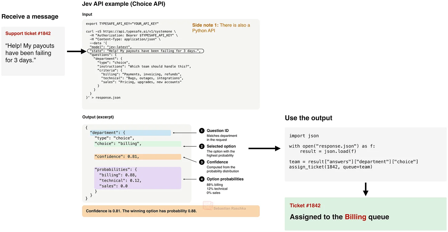
In short, there are three main API types illustrated below. Let’s start with the Choice API, which is convenient for multi-class classification.
Figure 25: Jev’s Choice API. Use this for multi-class classification.
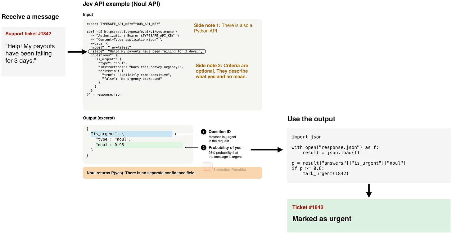
Next is the Noul API, which is simpler and assigns a “yes” probability to a question.
Figure 26: Jev’s Noul API. Use this for binary classification or multi-label classification (with multiple Noul questions).
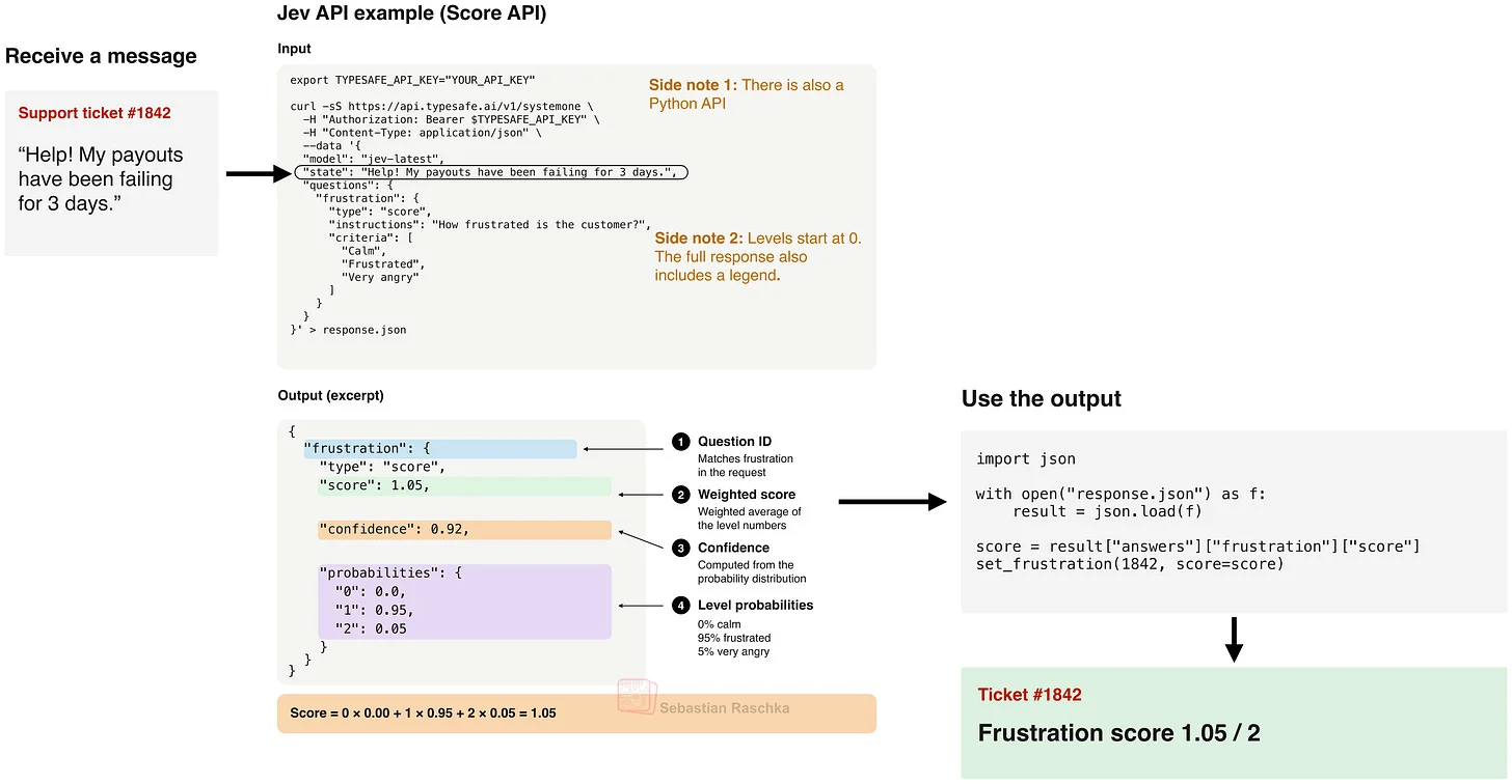
Lastly, the Score API assigns a score based on a rubric level (in the example below, 0, 1, 2).
Figure 27: Jev’s Score API. Use this for ordinal classification.
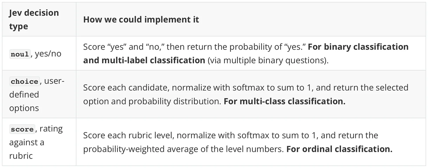
To sum it up, the different APIs and use cases are as follows.
Figure 28: Jev API cheat sheet.
过去几年,我们习惯了拿更大、更好、更贵的 GPT 式 LLM 砸各种问题。对有目标的决策/分类任务,Jev 这种便宜又快的东西让人耳目一新。尤其一次性任务,收集数据、微调 ModernBERT 太烦,直接扔个 Luna 类模型了事。
Jev 火不光因为通用(开箱在不同领域表现好),API 也确实好用,终端 curl 或 Python API 都能调。
简单说有三种 API,先看 Choice,适合多分类。
图 25:Jev 的 Choice API,用于多分类。
然后是 Noul,更简单,给一个问题返回“是”的概率。
图 26:Jev 的 Noul API,用于二分类或多标签分类(问多个 Noul 问题)。
最后是 Score,按评分规则(下例是 0、1、2 三档)打分。
图 27:Jev 的 Score API,用于有序分类。
总结,各 API 和用途如下。
图 28:Jev API 速查表。
【批注】 先把调用结构说白:state 是待判的文本,questions 是你要做的决策问题,criteria 是每个候选的自然语言描述——“任务说明 + 候选项”就装在这三个字段里。再释个词:ordinal classification(有序分类)指等级有顺序但间距不一定相等,比如 0/1/2 表示差/中/好,1 和 2 的差距不等于 0 和 1 的差距,所以 Score 的数字不能当刻度尺用。深一层看,Choice/Noul/Score 恰好对应测量学里的 nominal(二选多)/binary(是非)/ordinal(有序)三种量表,API 设计背后是经典测量理论,不是拍脑袋。工程上记住三条:Choice 的概率依赖候选集合,增删改写选项都会改变归一化结果;Noul 各问各的,不保证加起来等于 1;Score 的数字只在你定的规则里有意义。
3.3 拿 Jev 分类 IMDb
To make these APIs more concrete, and to answer the question of how well Jev might do on the aforementioned IMDb dataset, we can run it with either the Choice or Noul API.
Let’s start with the Choice API first. Each review would be formatted as follows:
This Choice API is convenient if we want to use explicit labels for binary (here) or multi-class problems.
An actual response might look as follows:
Along with the "choice": "positive" label, we also get the confidence for this prediction, which can be really useful in real-world applications, as well as the probabilities for each class. (The confidence field summarizes how concentrated the probability distribution is. It is different from the probability assigned to the winning class.) One of the selling points of Jev is that, according to the documentation, these are well-calibrated (but more on calibration later).
Alternatively, we can also use the Noul API here to classify the reviews. Using the same movie review classification context, the format would be as follows:
And the answer via the Noul API is:
(Interestingly, it gives 0.98 instead of 1.0 for the positive class, even though it’s the same text.)
We can also apply the Noul API to multiple classes by asking one question per class, for example:
- “Is this article about finance?”
- “Is this article about politics?”
- “Is this article about technology?”
Here, each question (independently from each other) returns a probability, and these probabilities don’t have to sum to 1. So, for a multi-class classification where each text can have multiple labels, we may prefer Noul, and for classification problems with only one final answer, Choice adds more convenience.
Now, running Jev with either Choice or Noul on the 25,000 movie reviews on the test set gave the following results:
- Choice:
- Accuracy 96.47% (24,117 correct)
- Total runtime: 22 minutes 24 seconds
- 15,456,663 input tokens, $0.6492 total cost
- Noul:
- Accuracy 96.20% (24,050 correct)
- Total runtime: 23 minutes 3 seconds
- 15,106,663 input tokens, $0.6345 total cost
Note that the small difference in performance and runtime between Choice and Noul could be due to random fluctuation since, similar to other LLMs, the runs are not fully deterministic.
For instance, I ran the Choice API a second time over the same test set and got slightly different results, as shown below.
Figure 29: Repeated Jev runs.
(The non-determinism when serving LLMs and other models at scale is likely due to batch-dependent GPU kernel execution changing the order of floating-point operations, as laid out in a nice blog post by Horace He last year.)
Anyways, the results look quite good overall (caveat: we don’t know if the IMDb test set was part of the training set).
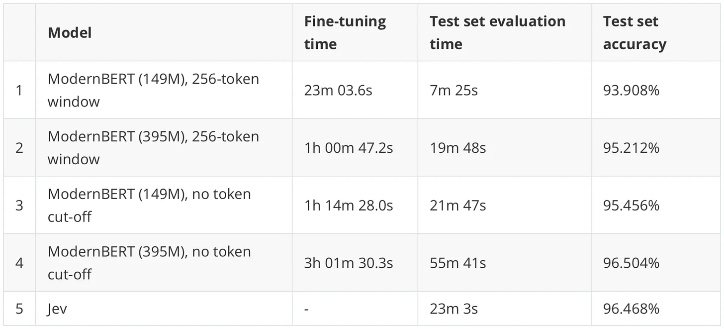
For reference, a ModernBERT model took
- 23 min to fine-tune on the training set;
- 7 min to evaluate on the test set.
For comparison, the best ModernBERT model has similar accuracy, as shown below (I expect you can still get 1-2% higher accuracy with additional hyperparameter tuning). Note that this was run on a DGX Spark, and it’s possible to get faster inference performance with quantization and faster hardware.
Figure 30: ModernBERT versus Jev.
But our ModernBERT model can’t play Tetris, for example, or do anything else besides movie classification without us fine-tuning it for the new task. But we could then throw a GPT-5.6 Luna or GPT-6 Luna model at it (which is a bit slower and also more expensive).
A classic rule of thumb was:
- Use a cheap LLM (like GPT-6 Luna) for one-off decision-making tasks;
- Fine-tune a custom classifier if we want to do this task repeatedly.
Now, something like Jev could take the place of the above to a) reduce latency and save money over Luna and b) save us the work of fine-tuning a custom model. (Although if we have a very high-volume task and we want to maximize speed and accuracy on a very specific task, it, of course, still makes sense to fine-tune.)
为了让这些 API 更具体,也回答 Jev 在前面说的 IMDb 数据集上到底如何,我们分别用 Choice 和 Noul 跑一遍。
先看 Choice,每条影评的调用格式如下(见下方 curl,state 是影评文本,questions 里定义 sentiment 选择题,criteria 给出 negative/positive 的自然语言描述)。
Choice 适合想用显式标签的二分类(本例)或多分类问题。
实际返回大概长这样(见下方 JSON):choice 为 positive,confidence 1.0,各类 probabilities,以及 token 用量。
除了 "choice": "positive" 标签,还拿到这次预测的 confidence(实际应用里很有用),以及每个类的概率。(confidence 字段概括的是概率分布有多集中,和胜出类的概率不是一回事。)Jev 的卖点之一是:按文档说法,这些概率是良好校准的(校准后面细说)。
也可以用 Noul 给影评分类,同样语境下格式如下(见下方 curl:问 “is_positive”,类型 noul)。
Noul 的回答如下(见下方 JSON):"noul": 0.98。
(有意思的是,同一段文本,Noul 给正类 0.98 而不是 1.0。)
Noul 也可以一类一问地用到多类上,例如:
- “这篇文章讲金融吗?”
- “这篇文章讲政治吗?”
- “这篇文章讲技术吗?”
每个问题各自独立返回一个概率,这些概率加起来不必等于 1。所以,一篇文本可属多个标签的多分类用 Noul 更合适;只要一个最终答案的分类问题,Choice 更方便。
现在,在测试集 25,000 条影评上跑 Jev,Choice 和 Noul 的结果如下:
- Choice:
- 准确率 96.47%(答对 24,117)
- 总耗时 22 分 24 秒
- 输入 token 15,456,663,总费用 $0.6492
- Noul:
- 准确率 96.20%(答对 24,050)
- 总耗时 23 分 3 秒
- 输入 token 15,106,663,总费用 $0.6345
注意 Choice 和 Noul 在性能和耗时上的小差异可能是随机波动,和其他 LLM 一样,多次运行不完全确定。
比如,我把 Choice 在同一测试集上又跑了一遍,结果略有不同,如下图。
图 29:重复运行 Jev。
(大规模 serving 时 LLM 和其他模型的非确定性,大概率是因为 batch 相关的 GPU kernel 执行改变了浮点运算顺序,Horace He 去年有篇不错的博客讲这个。)
总之结果整体很好看(提醒:我们不知道 IMDb 测试集进没进过训练集)。
对照一下,ModernBERT 模型花了:
- 23 分钟在训练集上微调;
- 7 分钟在测试集上评估。
对比,最好的 ModernBERT 模型准确率相近,如下图(再调调超参估计还能涨 1-2 个点)。注意这是在 DGX Spark 上跑的,量化和更好的硬件还能更快。
图 30:ModernBERT vs Jev。
但我们的 ModernBERT 模型不会玩俄罗斯方块,不微调的话除了影评分类啥也干不了。这时可以扔 GPT-5.6 Luna 或 GPT-6 Luna 上(慢一点,也贵一点)。
经典经验法则是:
- 一次性决策任务,用便宜的 LLM(如 GPT-6 Luna);
- 要反复做的任务,微调专用分类器。
现在,Jev 之类的东西可以取代上面两条:a)比 Luna 延迟更低、更省钱;b)省掉微调专用模型的活。(当然,如果是超高频任务,又想在特定任务上把速度和准确率拉满,微调还是有意义的。)
【批注】 先把”便宜”翻译成体感:$0.65 跑 2.5 万条,单条约 0.0026 美分(不到人民币 0.0002 元);22 分钟跑完是 API 并发下的吞吐(约每秒 19 条),不是单条延迟——延迟看 Tetris 视频那个实时演示。另释个词:non-determinism 那段引的 Horace He 博客,意思是 batch 不同会导致 GPU 浮点加法顺序不同,所以同 prompt 两次结果有零星出入,这不是 Jev 的 bug,是大规模 serving 的通病。动机上注意一点:作者主动说出”不知道 IMDb 测试集进没进训练集”——这是可信度操作,替读者把最狠的质疑先说了。数字的边界也要摆正:这是作者一套调用设置下的结果,不能证明训练测试隔离,不代表中文/多语言/高风险场景,更代替不了跨领域评测;真要评估通用决策能力,还得查候选措辞变化、类别分布变化、分布外输入、校准误差、重复性和误判成本。
1 | export TYPESAFE_API_KEY="YOUR_API_KEY" |
1 | { |
1 | curl -sS https://api.typesafe.ai/v1/systemone \ |
1 | { |

4. 给 BERT/GPT 式模型套上 Jev 式 API
Of course, we could also be adding a Jev-like API on top of a (Modern)BERT or any GPT-style model. Adding a Jev-like API is pretty straightforward. In fact, as soon as Jev was released, I built a Jev-like ModernBERT model to show how simple it is to build your own Jev model.
I decided not to release my Jev clone because I changed my mind in the meantime. I.e., it’s trivial to put a Jev-like API on top of ModernBERT, and it’s trivial to fine-tune it on a bunch of classification tasks. But it’s not trivial to make this model work well on all different kinds of tasks (like Tetris) without extensive training and testing. (Also, there are already enough quick Jev clones riding on the hype train by now; the world doesn’t need another quick clone, but a strong open-weight version would be nice, of course.)
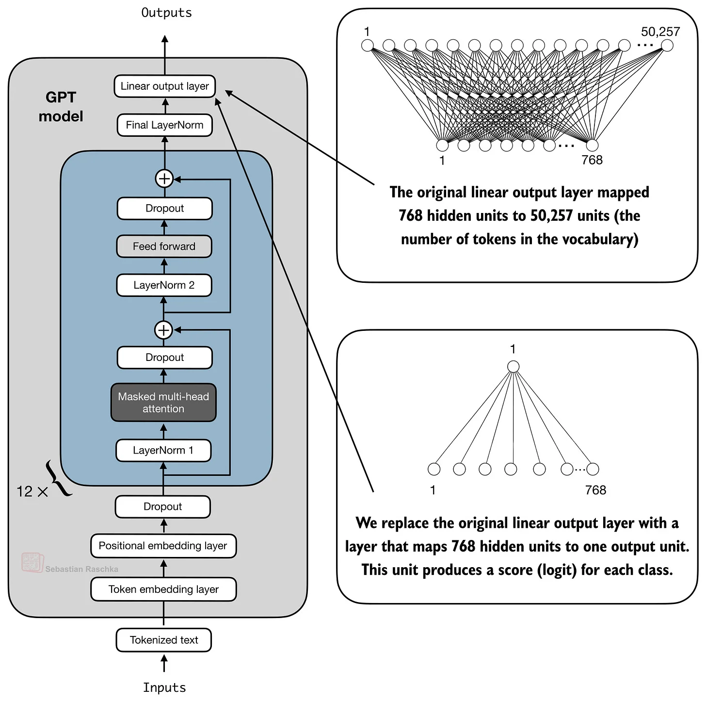
However, if you are interested in how that retrofitting would work, here is a quick overview. For example, we can implement a Jev-like Choice API by adding a small classification head to any BERT-, GPT-, or T5-style model as illustrated earlier. But instead of having the output nodes in this head match the number of classes, we have it with only 1 output node, as illustrated for the modified GPT model below.
Figure 31: GPT model where we replace the output layer (which maps to the whole vocabulary) with an output head with only one node.
Earlier, we discussed fine-tuning these models for a specific task like movie review classification with a pre-defined number of class labels (here, “positive” and “negative”). With this “1 output node” setup, we can actually extend this to a flexible and arbitrary number of classes.
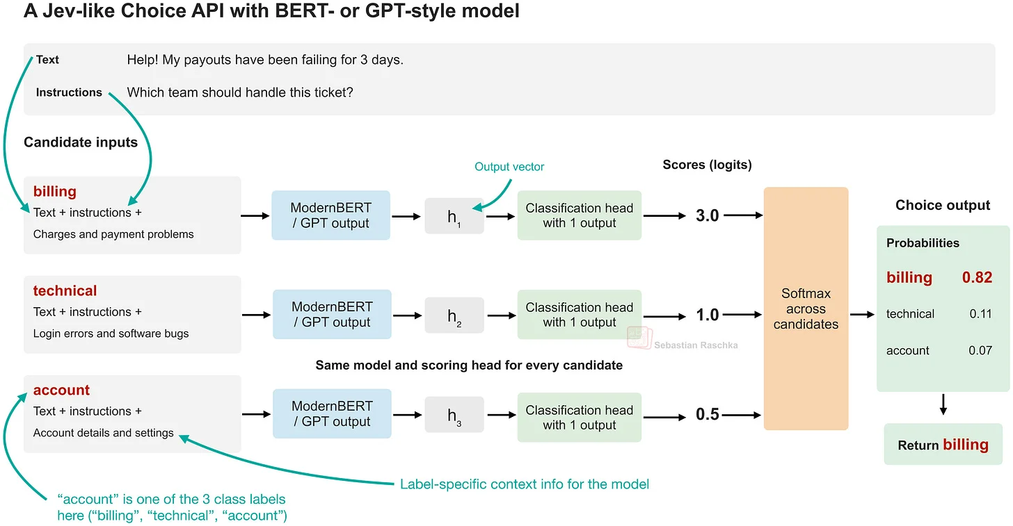
To extend this to an arbitrary number of classes (let’s consider the 3-class case of categorizing a customer ticket into the three categories “billing”, “technical”, “account”), we can do so as shown in the figure below.
Figure 32: Using a BERT- or GPT-style model with a Jev-like choice API.
As shown in the figure above, for each candidate option, we feed the model the input text, the task instructions, and the candidate’s description. The classification (scoring) head maps the output representation to a single scalar score. We then apply softmax across the candidate scores to obtain a probability distribution and return the highest-probability option.
The main point here is that the proposed head has one output per class. Each class description produces its own representation, which the same head scores via the output layer (which is essentially a logistic regression model): a scalar score per candidate computed from a learnable weight, a learnable bias, and the transformer’s output representation before the classification head (the original article shows this as a formula illustration), where
- s_i is the scalar score for class label i;
- w is a learnable weight;
- b is a learnable bias unit;
- h_i is the output of the transformer before the classification head.
For N candidates, this produces N scores. Softmax then returns N probabilities. The learned parameters stay the same when N changes.
Note that for h_i:
- BERT-style encoder models use the final hidden state of the
[CLS]token (optionally passed through a pooling layer); - GPT-style autoregressive models typically use the final non-padding token’s hidden state, which we need because of the autoregressive nature as discussed earlier (the last non-padding token can attend to the preceding text, instructions, and candidate description).
Then, we fine-tune the model and the scoring head jointly using cross-entropy loss against the correct option. Since all candidates share the same scoring head, we can change the number and descriptions of the options without changing the architecture. But again, how well this works on unfamiliar tasks depends on the training data.
By the way, why BERT- or GPT-style transformer-based models over simpler RNN and CNN architectures mentioned earlier? From a technical perspective, the approach outlined above works with either. But transformer-based models scale really well, meaning they can be pre-trained on larger datasets and benefit more than other models. Also, they can make good use of the information provided in the context (thanks to attention). So, if we want our model to generalize well to different target tasks without explicit fine-tuning on each one, pre-training a transformer-based model on a high-quality dataset likely gets us closer than RNN- or CNN-based models.
当然,也可以给 (Modern)BERT 或任何 GPT 式模型套个 Jev 式 API。套 API 本身很简单。事实上 Jev 一发布,我就搭了个 Jev 式 ModernBERT,演示自己造 Jev 有多简单。
但我后来改主意了,没发布这个克隆:给 ModernBERT 套 Jev 式 API 是小事,在一堆分类任务上微调也是小事;难的是不经过大量训练和测试,就让它在各种任务(比如俄罗斯方块)上都好用。(再说蹭热度的速成克隆已经够多了,世界不需要再多一个,但一个强的开源版本当然欢迎。)
不过如果你想知道这个改造怎么做,这里快速讲一遍。比如,给任意 BERT/GPT/T5 式模型加个小分类头,就能实现 Jev 式 Choice API(前面图解过)。但这个头的输出节点数不再等于类别数,而是只有 1 个输出节点,下图是改造后的 GPT 模型。
图 31:把输出层(映射到全词表)换成只有 1 个节点的输出头的 GPT 模型。
前面讲过给特定任务(如影评分类,类别数预先定好:”positive”/“negative”)微调这些模型。用“1 个输出节点”这套,可以扩展到灵活、任意数量的类别。
扩展到任意数量类别(比如客服工单分 3 类:”billing””technical””account”),做法如下图。
图 32:给 BERT/GPT 式模型套 Jev 式 choice API。
如上图,对每个候选项,把输入文本、任务说明和该候选的描述一起喂给模型。分类(打分)头把输出表示映射成一个标量分数,然后在所有候选分数上做 softmax 得到概率分布,返回概率最高的选项。
要点是:这个头对每个类只出一个数。每个类的描述各自产出一个表示,同一个头经输出层(本质上就是个逻辑回归)打分:每个候选的标量分由可学习的权重、可学习的偏置和分类头之前的 Transformer 输出表示算出(原文这里是个公式图),其中
- s_i 是类别标签 i 的标量分;
- w 是可学习的权重;
- b 是可学习的偏置;
- h_i 是分类头之前的 Transformer 输出。
N 个候选就产出 N 个分数,softmax 返回 N 个概率。N 变化时,学到的参数不变。
注意 h_i 的取法:
- BERT 式 encoder 模型用
[CLS]token 的最后隐状态(可选过一个池化层); - GPT 式自回归模型通常用最后一个非 padding token 的隐状态——自回归的性质决定了必须这样(前面讲过:最后一个非 padding token 能看到前面的文本、说明和候选描述)。
然后,用交叉熵损失对着正确选项,把模型和打分头一起微调。所有候选共享同一个打分头,所以换选项数量、改选项描述都不用改架构。但还是那句话:在没见过的任务上好不好使,看训练数据。
顺带一问:为什么用 BERT/GPT 式 Transformer,而不用前面讲的更简单的 RNN/CNN?技术上说,上面这套两种都能搭。但 Transformer 扩展性好,能在更大数据集上预训练、吃到更多红利;还能用好上下文里的信息(靠 attention)。所以,如果想让模型不逐个微调就泛化到不同目标任务,在高质量数据集上预训练 Transformer 大概率比 RNN/CNN 走得更远。
【批注】 把”接口通用”的数学实质说透:传统分类头的输出维度 = 类别数,换任务(比如从 2 类变 3 类)就得换头重训;Jev-like 的头永远只输出 1 个数,类别变化只改输入文本、不改架构——通用性就藏在这里。再补个呼应:h_i 取法那段(BERT 取 [CLS]、GPT 取最后一个 token)把 2.1、2.2 全串起来了,这一章是上篇的收束,读的时候要往回看。billing/technical/account 那个例子也别当随意举例,工单三分类正是 Jev 最典型的真实用例(前文 support tickets 就提过)。但架构通用 ≠ 自动理解新任务:候选描述清不清楚、候选覆没覆盖全、训练时见没见过类似任务,都会影响输出,可靠性还得靠任务数据和系统评测。
作者也明确区分“做出相似 API”与“训练出同等泛化能力”:接口容易模仿,支撑模型表现的数据、训练流程和评测体系并不会随 API 一起复制。
【批注】 “trivial to build API, nontrivial to generalize” 是全文金句,动机是双重的:给满屏的速成克隆泼冷水(接口长得像 ≠ 泛化一样),同时把悬念抬给第 5 章——既然接口不值钱,那值钱的就是数据和训练。演示里某个模型能调 Choice,只能证明接口抄对了,泛化范围得看多任务实测。所以读第 6 章那些克隆(CLM 82.9%、Laya 92.33%)时,IMDb 数字好看不算数,Tetris 那种没见过的任务才是试金石。
5. Jev 的架构与训练算法
So, how come Jev does so well on so many different tasks (from movie reviews to something arbitrary like playing Tetris)? Unfortunately, the architecture, algorithm, and training data details are not public. Also, keep in mind there’s a whole team and multi-million-dollar company behind it that specialized in and worked really hard on this model; we can’t expect to match that level of performance by training a ModernBERT-like model for a week on some open datasets.
That being said, if I had to make an educated guess, architecture-wise, I’d guess that they are using something small similar to ModernBERT, hence, the low latency.
For the training data, as mentioned before, the TypeSafe AI CEO said the following:
100% of our data is synthetic (but not the type of crap that is just spit out from an LLM obviously)
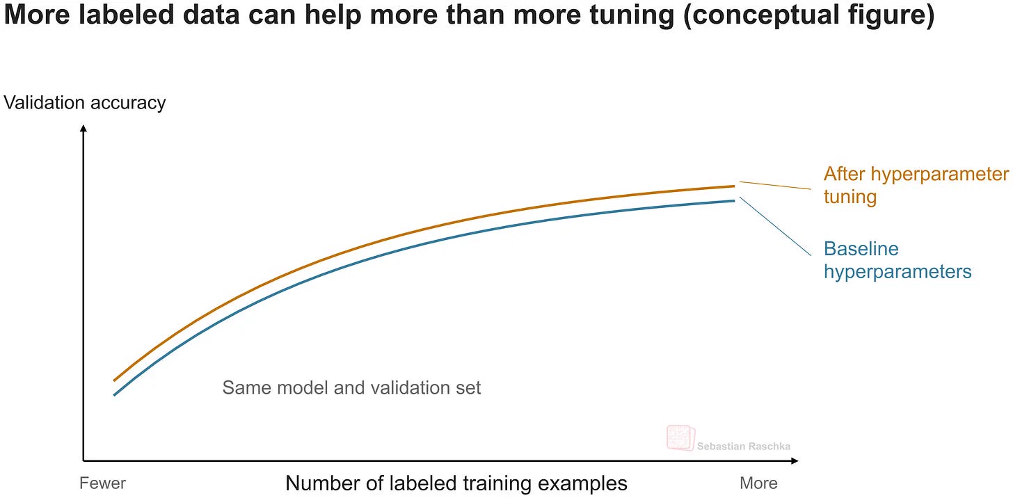
So, yeah, I think most of the effort went into curating this dataset. It’s something I’ve also been preaching to students and collaborators for many years. As a short anecdote, about 8 years ago, I was collaborating with another professor in the social sciences department and helped to design the experimental setup for a text classification problem. Her student spent many days hyperparameter tuning both a bag-of-words baseline and a BERT model to eke out ~2-5% accuracy. Then I suggested we each sit down for a few days to hand-label more data (I think our original dataset was around 300 samples, and we doubled the size), which resulted in a >10-20% accuracy boost. Yes, it’s important to plot learning curves for that purpose :).
Figure 33: Rule of thumb showing that often more data helps more than additional hyperparameter tuning.
Finally, the training algorithm. Again, the details are not known, but TypeSafe AI’s blog post states that they were using a new algorithm called Reinforcement Learning for Calibrated Decisions (RLCD):
“We built a new stack entirely focused on automation: with a new model architecture, parallel sampler for maximum efficiency, and training method we call Reinforcement Learning for Calibrated Decisions (RLCD).”
This method is not public. A published method with a similar calibration objective is RLCR (Reinforcement Learning with Calibration Rewards), from the 2025 paper Beyond Binary Rewards: Training LMs to Reason About Their Uncertainty. Before providing more details, the next section gives a brief overview of calibration in general.
那么,Jev 为什么在这么多不同任务上(从影评到俄罗斯方块这种八竿子打不着的)都这么好?遗憾的是架构、算法、训练数据细节都不公开。也要记住背后是一整个团队、一家几百万美元的公司,专门死磕这个模型;别指望拿 ModernBERT 之类的在公开数据集上训一周就追上。
话虽如此,如果非要做有根据的推测,架构上我猜是 ModernBERT 之类的小东西,所以延迟低。
训练数据方面,前面提过,TypeSafe AI 的 CEO 说:
100% of our data is synthetic (but not the type of crap that is just spit out from an LLM obviously)
(我们的数据 100% 是合成的——但显然不是 LLM 随口吐的那种垃圾。)
所以我觉得主要功夫花在清洗这份数据集上。这也是我多年来一直跟学生和合作者念叨的。讲个小故事:8 年前我和社科系一位教授合作,帮她设计一个文本分类问题的实验。她学生花了很多天调词袋基线和 BERT 的超参,抠出 ~2-5% 的准确率。后来我建议大家各坐下来几天,多手标点数据(原始数据集大概 300 条,我们翻了一倍),结果涨了 >10-20%。所以,画学习曲线真的很重要(plot learning curves)。
图 33:经验法则——加数据常常比加调参更有用。
最后是训练算法。细节同样未知,但 TypeSafe AI 的博客写道,他们用了一种叫 Reinforcement Learning for Calibrated Decisions(RLCD,面向校准决策的强化学习)的新算法:
“We built a new stack entirely focused on automation: with a new model architecture, parallel sampler for maximum efficiency, and training method we call Reinforcement Learning for Calibrated Decisions (RLCD).”
(“我们搭了一套完全为自动化而生的新栈:新模型架构、为最高效率设计的并行采样器,以及我们称为 RLCD 的训练方法。”)
这个方法不公开。目标类似的已发表方法有 RLCR(Reinforcement Learning with Calibration Rewards,带校准奖励的强化学习),出自 2025 年论文 Beyond Binary Rewards: Training LMs to Reason About Their Uncertainty。讲细节之前,下一节先快速过一遍校准是什么。
5.1 关于校准
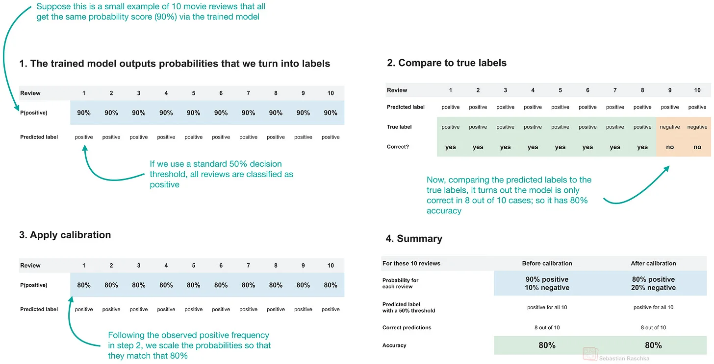
Calibration is not a new topic and a step I recommend for any production model where you want to use and evaluate the class-membership probabilities. In short, calibration adjusts the model’s probability estimates so they better match observed class frequencies.
For example, consider once more our IMDb movie classification problem. A model might assign a review 74% positive and 26% negative. These are probability estimates, but the model may be overconfident or underconfident. We cannot assume that the numerical values are reliable without evaluating calibration. I.e., predictions of 74% positive and 54% positive both yield the class label “positive” at a 50% threshold, although the model expresses more confidence in the 74% case.
Figure 34: Illustration of how calibration works.
Calibration techniques use a separate labeled dataset, e.g., a held-out validation set, to adjust these probability estimates. After successful calibration, among many reviews assigned a positive probability of approximately 74%, roughly 74% should actually be positive. For more information, I recommend the good old scikit-learn documentation.
There are many approaches for this. For example, one that I used in my AI detector project is temperature scaling. Temperature scaling divides the model’s logits by a temperature (T) value before applying softmax. We learn T (a positive number) by minimizing the cross-entropy loss on the calibration dataset while keeping the model weights fixed. A temperature above 1 reduces confidence in the highest-probability class, while a temperature between 0 and 1 increases it. We then use this same temperature for new predictions. Because this scaling preserves the ordering of the logits, the predicted class remains unchanged when we select the highest-probability class.
校准不是新话题,只要生产模型要用、要评估类别概率,我都建议做这一步。简单说,校准调整模型的概率估计,让它和观测到的类别频率对上。
再拿 IMDb 影评举例:模型给一条影评 74% positive、26% negative。这是概率估计,但模型可能过度自信也可能信心不足。不评估校准,不能默认这些数字靠谱。比如 74% positive 和 54% positive 在 50% 阈值下都判 “positive”,但模型对前者的信心表达强得多。
图 34:校准是怎么回事。
校准技术用一份独立的有标注数据集(比如留出的验证集)来调这些概率估计。校准成功后,被赋予约 74% 正类概率的一大批影评里,应该真有约 74% 是正类。更多资料推荐经典的 scikit-learn 文档。
办法很多。比如我在 AI detector 项目里用的温度缩放(temperature scaling):softmax 之前,把模型的 logits 除以一个温度值 T。固定模型权重,在校准数据集上最小化交叉熵损失,学出 T(正数)。温度大于 1 压低最高概率类的信心,0 到 1 之间则抬高。新预测沿用这个温度。因为缩放不改变 logits 的排序,取最高概率类时,预测类别不变。
5.2 带校准奖励的强化学习(RLCR)
Jev’s RLCD training method remains proprietary, but a related idea we can discuss is Reinforcement Learning with Calibration Rewards (RLCR), which was introduced in the 2025 Beyond Binary Rewards: Training LMs to Reason About Their Uncertainty paper. (Note that there is no officially established connection between the two methods, but I am assuming that they could be related.)
Reinforcement learning with verifiable rewards (RLVR) typically rewards a correct answer with 1 and an incorrect answer with 0. (For a comprehensive explanation and implementation, I recommend checking out my Build A Reasoning Model (From Scratch) book :)).
In short, RLCR adds an additional penalty for inaccurate confidence estimates.
So, in the conventional RLVR method, the reward R is either 0 or 1 based on the answer correctness (we are ignoring an optional formatting reward and length penalty here, for simplicity).
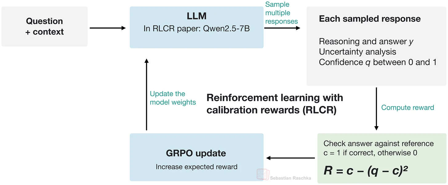
In RLCR, the model generates reasoning and an answer, which is followed by an uncertainty analysis and a numerical confidence (q). This modified reward is
where c is 1 for a correct answer and 0 otherwise. For example, an incorrect answer with 90% (0.9) confidence receives a reward of -0.81, since
At 20% confidence, the reward is -0.04. And a correct answer at 90% confidence earns 0.99. (Readers familiar with evaluating calibrated models may notice that the squared-error term is the Brier penalty for the stated probability that the answer is correct.)
Figure 35: RLCR overview.
Note that the same (here, Qwen2.5-7B) model generates the uncertainty analysis and q as part of its response.
The uncertainty analysis is a written assessment of where its answer could be wrong. After answering, the model examines missing evidence, ambiguous wording, questionable assumptions, or possible reasoning errors. The paper’s prompt asks it to identify specific uncertainties rather than propose corrections.
Also, the system prompt explicitly asks for q, a number between 0 and 1 inside tags. It represents the model’s estimated probability that its answer is correct. The system generates all these parts sequentially in the same response.
For illustration purposes, the model answer could be as follows:
2
3
4
5
6
<answer>positive</answer>
<analysis>
The passage mentions a positive movie review, but the connection to the second paragraph is unclear.
</analysis>
<confidence>0.6</confidence>
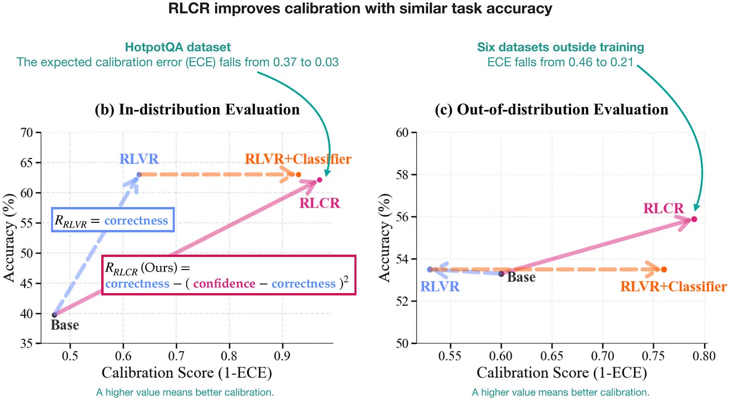
Below is an annotated figure from the paper that illustrates how it improves the expected calibration error over regular RLVR with temperature scaling.
On HotpotQA, RLCR reduces expected calibration error (ECE) from 0.37 to 0.03 compared with RLVR, with similar accuracy (62.1% versus 63.0%). Across six other datasets, average ECE falls from 0.46 to 0.21, while accuracy rises from 53.9% to 56.2%. These are the results in the paper’s Table 1(a).
Figure 36: RLCR results from the Beyond Binary Rewards: Training LMs to Reason About Their Uncertainty paper.
Conceptually, the “Classifier” in “RLVR + Classifier” is a supervised binary classifier that predicts whether the generated answer is correct.
For Jev, I could apply calibration rewards directly to typed decisions, without generating reasoning text. For example, we could equip a GPT-style model with the classification head illustrated in Section 2.2 and adapt the RL training objective to reward accurate decisions and calibrated probabilities. We would train the backbone and classification head together. This would be an adaptation inspired by RLCR, and it remains unclear whether Jev’s RLCD works this way.
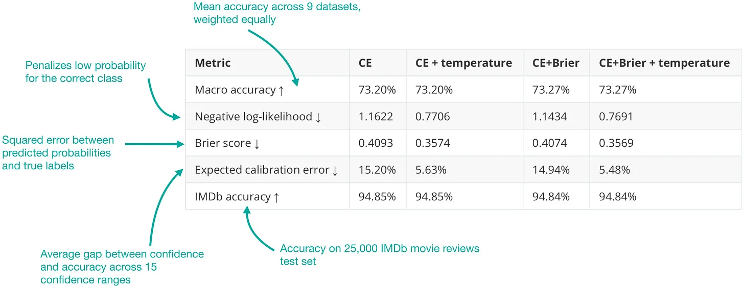
Alternatively, since Direct Policy Optimization (DPO) is a cross-entropy (CE) alternative to Reinforcement Learning with Human Feedback (RLHF), we could also directly minimize CE + Brier loss on the classifier’s probabilities. I did this with the ModernBERT model, and there was a modest improvement over regular temperature scaling.
Figure 37: ModernBERT improvements via RLCR-inspired Brier-loss optimization. The ↑ symbol means higher is better. The ↓ symbol means lower is better.
(For simplicity, the figure above only shows the average results over nine datasets. Overall, as can be seen, calibration was beneficial on average. However, it slightly worsened the ECE on one out of the nine datasets.)
Jev 的 RLCD 训练方法仍是私有的,但有个相关的思路可以聊:Reinforcement Learning with Calibration Rewards(RLCR,带校准奖励的强化学习),出自 2025 年论文 Beyond Binary Rewards: Training LMs to Reason About Their Uncertainty。(注意两者没有官方确认的联系,我只是推测它们可能相关。)
带可验证奖励的强化学习(RLVR)通常答对给 1、答错给 0。(全面讲解和实现推荐看我的 Build A Reasoning Model (From Scratch)。)
一句话:RLCR 对不准的置信度估计追加惩罚。
传统 RLVR 里奖励 R 按答案对错非 0 即 1(为简单起见,这里忽略可选的格式奖励和长度惩罚)。
RLCR 里,模型生成推理和答案,之后跟一段不确定性分析和一个数字置信度 q。改造后的奖励是
其中答案正确时 c=1,否则 c=0。比如答错但置信度 90%(0.9),奖励是 -0.81,因为
置信度 20% 时奖励是 -0.04。答对且置信度 90% 得 0.99。(熟悉校准模型评估的读者会发现,平方误差项就是对“答案正确”这一声称概率的 Brier 惩罚。)
图 35:RLCR 总览。
注意不确定性分析和 q 是同一个模型(这里是 Qwen2.5-7B)在回复里顺带生成的。
不确定性分析是书面评估“我的答案可能错在哪”。作答后,模型检查缺失证据、含糊措辞、可疑假设或可能的推理错误。论文的 prompt 要求它指出具体的不确定点,而不是提修改建议。
系统 prompt 还明确要求输出 q(标签里的 0 到 1 数字),表示模型估计自己答案正确的概率。所有这些部分在同一回复里顺序生成。
举例,模型回答可能是这样:
2
3
4
5
6
<answer>positive</answer>
<analysis>
The passage mentions a positive movie review, but the connection to the second paragraph is unclear.
</analysis>
<confidence>0.6</confidence>
下面是论文的注释版图,展示它相对普通 RLVR + 温度缩放,把期望校准误差降了多少。
HotpotQA 上,RLCR 把期望校准误差(ECE)从 0.37 降到 0.03,准确率相近(62.1% vs 63.0%)。另外六个数据集上,平均 ECE 从 0.46 降到 0.21,准确率从 53.9% 涨到 56.2%。这是论文表 1(a) 的结果。
图 36:Beyond Binary Rewards 论文的 RLCR 结果。
概念上,”RLVR + Classifier” 里的 “Classifier” 是个有监督二分类器,预测生成的答案对不对。
对 Jev,我可以把校准奖励直接用在类型化决策上,不生成推理文本。比如给 GPT 式模型装上 2.2 节图解的分类头,把 RL 训练目标改成奖励准确决策 + 校准概率,骨干和分类头一起训。这算是受 RLCR 启发的改编,Jev 的 RLCD 是不是这么干的,仍不清楚。
另一条路:Direct Policy Optimization(DPO)是 RLHF 的交叉熵(CE)替代方案,我们也可以直接在分类器概率上最小化 CE + Brier 损失。我在 ModernBERT 上试过,相对普通温度缩放有小幅提升。
图 37:受 RLCR 启发的 Brier 损失优化给 ModernBERT 带来的提升。↑ 越高越好,↓ 越低越好。
(为简单上图只展示了九个数据集的平均结果。整体看校准平均有益,但在一个数据集上 ECE 轻微变差。)
【批注】 先把公式翻译成人话:R = c - (q-c)² 里,答错时奖励恒 ≤0(最高 0,最低 -1),答对时恒 ≥0(最低 0,最高 1)——模型永远有动力先答对,同时不敢瞎自信。再释两个词:Brier score = 预测概率和 0/1 真实结果的均方误差,越小越校准;ECE(期望校准误差)= 按置信度分桶后,桶内准确率和平均置信度的差距加权平均,HotpotQA 上 0.37→0.03 就是这么来的。动机上要看穿作者的手法:RLCD 不公开,他拿最像的公开工作 RLCR 来”借尸还魂”推理,所以满篇限定词(assuming、remains unclear)——这是学术自保,读的时候把”厂商公开的 / 作者实测的 / 作者猜的”分三层放:RLCD 存在是厂商说的,Brier 加持有效是作者实测的,Jev 用 RLCD 是作者猜的。
原文对此的限定是:”there is no officially established connection between the two methods”(两种方法之间没有官方确认的联系)。
5.3 旁注:校准有必要吗
Cross-entropy already encourages accurate probability estimates. Under ideal conditions, that is enough to obtain calibrated predictions without an additional penalty.
I.e., using a simple coin flip example analogous to the movie review classification, the two classes are “heads” and “tails.” If it’s a biased coin that lands heads 80% of the time (in expectation), the true probabilities are 80% heads and 20% tails. On a representative training set, when we optimize cross-entropy, the model will already learn these as a side-effect of minimizing cross-entropy (negative-log-likelihood).
So, in short, if the model learns the true class probabilities, its predictions are calibrated and an additional penalty is unnecessary. (And Brier loss has the same theoretical optimum as cross-entropy, as described in Strictly Proper Scoring Rules, Prediction, and Estimation by Gneiting and Raftery, 2007.)
In practice, however, we never train to the real optimum (in expectation) but train on a finite dataset.
So, once a neural network correctly classifies most training examples, it can further reduce cross-entropy on the training set by becoming more confident. These confidence estimates may then generalize poorly to the test set and new data.
For example, in On Calibration of Modern Neural Networks, Guo et al. (2017) observed “neural networks can overfit to NLL without overfitting to the 0/1 loss.”
That means test accuracy can still improve while test cross-entropy worsens. So overfitting can show up in the probability estimates even when classification accuracy continues to improve.
Adding Brier loss changes how prediction errors are weighted during training. But whether this improves calibration needs to be checked on held-out data, of course. (The modest improvement in my experiment is an empirical observation for this setup, and we should not assume that adding Brier will always help.)
In my experiments (see previous figure), adding the Brier loss to cross-entropy provided only a very small additional calibration benefit.
But the motivation is more direct in RL contexts, such as described in RLCR, where we measure answer correctness and don’t already minimize cross-entropy. So, in RL contexts, the Brier term adds an incentive to report accurate confidence alongside the reward for answer correctness.
交叉熵本身就在鼓励准的概率估计。理想条件下,只靠它就足以得到校准好的预测,不需要额外惩罚。
打个比方,和影评分类类似的抛硬币:两类是“正面”“反面”。如果硬币有偏,期望 80% 出正面,真概率就是 80% 正、20% 反。在有代表性的训练集上优化交叉熵时,模型最小化交叉熵(负对数似然)的副产品就是学会这两个数。
所以一句话:如果模型学到了真实类别概率,它的预测就是校准的,额外惩罚没必要。(Brier 损失和交叉熵理论最优点相同,见 Gneiting 和 Raftery 2007 年的 Strictly Proper Scoring Rules, Prediction, and Estimation。)
但实践中我们永远训不到真正的(期望)最优,只在有限数据集上训。
神经网络分对大多数训练样本后,还能靠变得更自信继续压低训练集交叉熵。这些置信度估计在测试集和新数据上可能泛化很差。
比如 On Calibration of Modern Neural Networks 里 Guo 等人(2017)观察到 “neural networks can overfit to NLL without overfitting to the 0/1 loss”(神经网络可以只对 NLL 过拟合,而不对 0/1 损失过拟合)。
意思是测试准确率还在涨,测试交叉熵却在变差。所以过拟合可以藏在概率估计里,即使分类准确率还在提升。
加 Brier 损失改变了训练时预测误差的加权。但能不能改善校准,当然要在留出数据上验证。(我的实验里那点小提升只是这套设置的经验观察,不能默认加 Brier 永远有帮助。)
我的实验里(见上图),交叉熵上加 Brier 只带来很小的额外校准收益。
但在 RL 场景下动机更直接,比如 RLCR:那里只量答案对错,本来就不最小化交叉熵。所以 RL 里 Brier 项给“报准置信度”加了个激励,和“答案正确”的奖励并列。
6. Jev 适合谁
Now that we covered Jev in reasonable detail, who is Jev for? Based on my assessment, it’s a pretty big target audience that intersects between people who a) want to save time by not having to fine-tune a custom classifier for every decision task and b) want to save money over using “the big guns” like GPT-6 and similar LLMs.
There are also lots of interesting use cases to think of. In the section below is a short list of ideas.
Jev 已经讲得够细了,那么它适合谁?按我的评估,目标人群不小,是两类人的交集:a)不想给每个决策任务微调专用分类器、想省时间的人;b)不想用 GPT-6 这类“重炮”LLM、想省钱的人。
有意思的用例也很多,下面是个简短的点子清单。
6.1 Jev 的用例
The list of use cases is seemingly endless. Sure, there are flashy examples like having it play video games like Tetris (as I showed in my earlier video above to demonstrate the low latency of the API). However, sorting emails is a more practical choice for most. For example, one could use Jev as an additional spam filter, prioritization, and so on.
But beyond things like that, it could also serve as a tool to augment LLM-agent harnesses. Here it could be used as
- a pre-screener for regular LLM-agent harnesses to scan our contexts for prompt injection;
- select the reasoning effort level for a model;
- select a skill.md from your registered skill library;
- use it as a judge for evaluation or self-refinement;
- find relevant files for context building.
The list is practically endless. Someone even posted a survey on arXiv analyzing 2,170 Jev-related projects that have sprung up recently in just a few days.
用例清单似乎无穷无尽。玩俄罗斯方块这种是吸睛的例子(我前面视频里用它演示 API 低延迟),但对多数人,分邮件更实用。比如拿 Jev 当追加的垃圾过滤、优先级排序等等。
除此之外,它还能增强 LLM-agent harness,比如用来:
- 给常规 agent harness 做前置筛查,扫描上下文里的提示注入;
- 给模型选推理用力档位;
- 从注册的 skill 库里选 skill.md;
- 当评测或自我改进的裁判;
- 找相关文件来组装上下文。
清单实际上列不完。甚至有人在 arXiv 上发了篇survey,分析了短短几天冒出来的 2,170 个 Jev 相关项目。
【批注】 五个用例里”选 skill.md”最值得多看一眼——这正是 Agent harness(Claude Code 那套 skills 机制)的真实痛点:skill 路由。作者 9 月底就写这个,说明他已经在用 skill 机制想事了。另外”几天冒出 2170 个项目”是有出处的(arXiv 2609.30216),热度是量化过的,不是修辞。动机上注意作者的搭配:Tetris 是秀延迟(flashy),筛邮件是秀实用(practical),一 flashy 一 practical,两种读者都留住。定位上别当验证过的结论:决策服务更现实的姿势是先做便宜筛选、难例回退强模型,账要算漏报、误报、额外延迟和回退策略;提示注入筛查尤其不能靠单一置信度阈值做安全保证。
6.2 Jev 克隆和本地 Jev
Since Jev’s launch, 100s, if not 1000s, of quick Jev clones have sprung up. Most of the ones I checked out were just quick examples fine-tuning a ModernBERT or Qwen model with SFT and adding a Jev-like API.
Based on what I can tell, none of them achieves the same level of performance as Jev on such a breadth of tasks. Comparing these projects to Jev is like comparing Alpaca (the early instruction-finetuned LLM based off of the original LLaMA open-weight model) to GPT-6. Sure, it may work similarly in spirit, but your mileage will vary on real-world tasks.
No offense, but they seem like quick projects to jump on the hype train, and I don’t want to plug a specific one here.
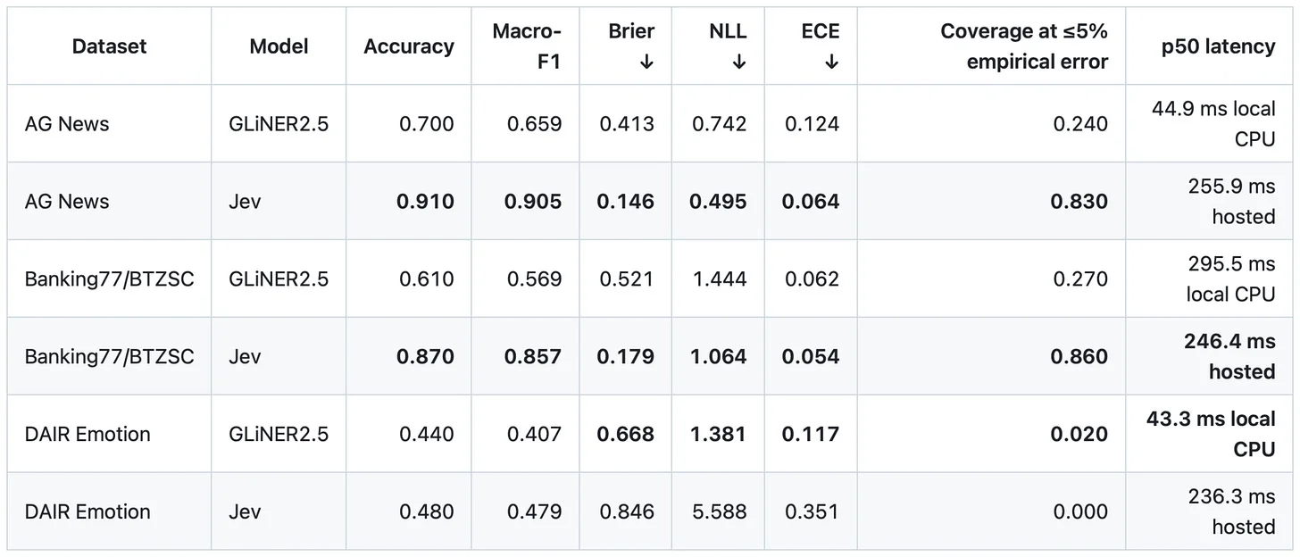
One exception here might be the GLiNER project, which has been around for ~3 years ago, and while it’s not fundamentally the same, it can be used for similar things. However, based on a benchmark, Jev is definitely stronger.
Figure 38: GLiNER vs Jev comparison via https://github.com/AbdelStark/jev-benchmarks/blob/main/results/reports/btzsc-pilot-v1.md
Anyways, there is definitely a genuine need and desire for a good open-weight alternative to Jev. The reason is not necessarily cost (because Jev is so cheap) but privacy. (Also, if Jev is already that fast over the internet, imagine how fast it could be on beefy local hardware.)
So, of course I’d like a DeepSeek (or Kimi, or GLM, or MiMo) moment for Jev. I am sure people are working on this, but it will take some time. TypeSafe AI worked on this for many months with a dedicated team of experts. It’s unrealistic to expect to replicate that development and evaluation work in a week. (However, since this is a smaller and more efficient model than a 1-trillion-parameter model, by nature, it hopefully won’t take that long.)
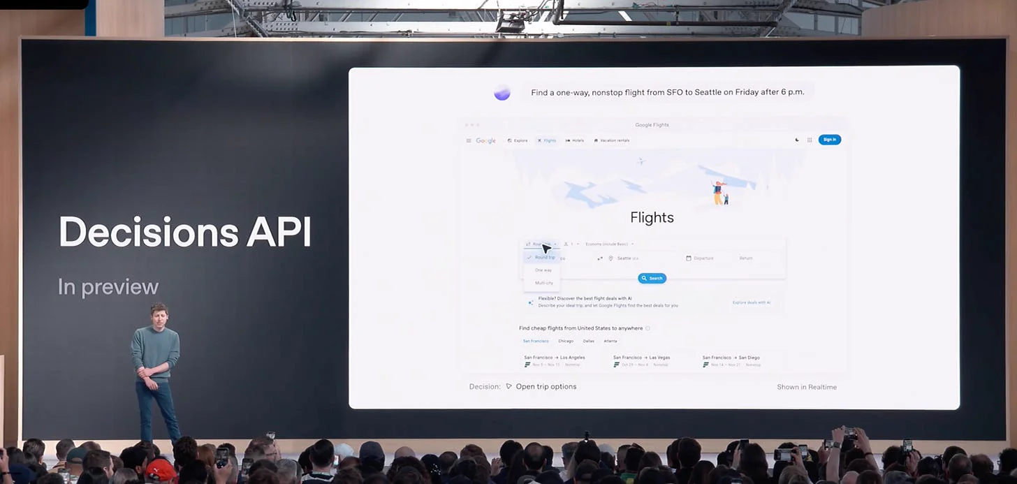
Update 1 (29 September, 10:20 am PT): OpenAI just announced the Decision API at their DevDay 2026 conference (29 September). It appears to be a Jev-like model directly integrated into their platform.
Decisions API enables real-time decision-making by focusing Luna’s intelligence on a specific set of user-defined questions with finite pre-defined answers. Developers supply context using text or images, and get back answers they can use to classify content, route requests, or choose an agent’s next action.
Available in limited preview today with a broad release planned in the coming days.
Figure 39: OpenAI’s Jev-like Decision API announced at the OpenAI Dev Day.
Update 2: A reader shared the Contrastive Language Models project with me in the comments below. It’s one of the nicer-looking Jev-likes. When I tried it, its IMDb test accuracy is just 82.90% (over 96.47% in Jev), and it fails the Tetris test.
Another reader wrote in about Laya, another strong contender. It did better at IMDb (92.33% test accuracy) but then failed the Tetris test even worse.
So, my point still stands. There are many solid alternatives. But what makes Jev so popular is not a unique idea (as mentioned before, classifiers existed for a long time) but the fact that it performs so well at so many diverse tasks. The only task where it allegedly doesn’t do well (as a reader told me) is legal reviews in non-English languages. (But the weak multilingual performance can be circumvented by connecting it to a cheap translation model, e.g., GPT-6 Luna with a small latency overhead.)
Jev 发布以来,冒出几百甚至几千个速成克隆。我看过的大多是拿 ModernBERT 或 Qwen 做 SFT 微调、再套个 Jev 式 API 的快餐例子。
就我所见,没有一个在这么广的任务面上达到 Jev 的性能。拿这些项目和 Jev 比,就像拿 Alpaca(基于原始 LLaMA 开源模型微调指令的早期 LLM)和 GPT-6 比:神似,实际任务上效果天差地别。
无意冒犯,但它们看着就是蹭热度的快项目,这里我不想点名推任何一个。
例外可能是 GLiNER,做了约 3 年了,虽然原理不完全一样,但能干类似的事。不过按这份 benchmark,Jev 明显更强。
图 38:GLiNER vs Jev 对比,数据见 jev-benchmarks。
总之市场确实真心想要个好的开源平替,理由不一定是钱(Jev 已经很便宜),而是隐私。(再想想:Jev 走互联网都这么快,上 beefy 本地硬件得快成什么样。)
所以我当然期待 Jev 的 DeepSeek(或 Kimi、GLM、MiMo)时刻。肯定有人在搞,但得花时间。TypeSafe AI 可是专家团队搞了好几个月,指望一周复刻人家的开发和评测工作不现实。(不过既然这是个更小更高效的模型,不像 1 万亿参数大家伙,希望不用等太久。)
更新 1(9 月 29 日上午 10:20 PT): OpenAI 在 DevDay 2026(9 月 29 日)刚发布了 Decision API,看着就是直接集成进自家平台的 Jev 式模型。
Decisions API enables real-time decision-making by focusing Luna’s intelligence on a specific set of user-defined questions with finite pre-defined answers. Developers supply context using text or images, and get back answers they can use to classify content, route requests, or choose an agent’s next action.
Available in limited preview today with a broad release planned in the coming days.
(Decision API 把 Luna 的智能聚焦到一组用户自定义的、答案有限预定义的问题上,实现实时决策。开发者用文本或图像提供上下文,拿回可用于内容分类、请求路由或选择 agent 下一步动作的答案。今日起限量预览,几天内全面发布。)
图 39:OpenAI 在 Dev Day 上发布的 Jev 式 Decision API。
更新 2: 有读者在评论区分享了 Contrastive Language Models,是长得比较顺眼的 Jev-like 之一。我试了下,它 IMDb 测试准确率只有 82.90%(Jev 是 96.47%),俄罗斯方块测试也没过。
另一位读者推荐了 Laya,另一个有力竞争者。IMDb 更好(92.33% 测试准确率),但俄罗斯方块测试挂得更惨。
所以我的观点不变:像样的替代不少,但 Jev 火不是因为点子独一无二(前面说了,分类器早有了),而是它在这么多不同任务上都很好。唯一据说不行的(一位读者告诉我的)是非英语的 legal review。(多语言弱可以用便宜翻译模型绕过去,比如 GPT-6 Luna,加一点延迟。)
Conclusion(原文结论)
All in all, at first glance, Jev doesn’t seem to offer anything fundamentally new. After all, one might say that “it’s just a classifier” (with a nice API on top of it). However, it works surprisingly well across a huge range of tasks. In that sense, it’s the plug-and-play version of dedicated classifiers.
Sure, experts will still fine-tune specialist models, but the bar to justify fine-tuning a specialized model is now much higher, since it’s easy to just throw a Jev or Jev-like at it and get good-enough results.
Also, I don’t expect Jev and Jev-likes to unlock new capabilities or solve previously unsolvable tasks. However, if we make such models part of our agent harnesses to aid the expensive GPT-6 or Opus 5.5 models in decision-making within that harness, using agent harnesses could become much faster and cheaper in the future.
总之,第一眼看 Jev 好像没啥根本性新东西,确实可以说“它就是个分类器”(套了个好用的 API)。但它在超广的任务面上好得出人意料,从这个意义上,它是专用分类器的即插即用版。
专家当然还会微调专用模型,但证明“值得微调”的门槛现在高多了——扔个 Jev/Jev-like 上去拿个够用的结果太容易了。
我也不指望 Jev 和 Jev-like 解锁新能力或解决以前解不了的任务。但如果把这类模型做进 agent harness,帮贵的 GPT-6 或 Opus 5.5 做 harness 内的决策,未来的 agent harness 会快得多、便宜得多。
总评:看决策接口,也看它的证据边界
这篇文章把文本分类的历史、Jev 的 API、作者实验和概率校准放在同一条线上。最值得带走的判断是:决策模型试图覆盖“任务很多、每个任务数据不多、又不想维护一套专用分类器”的需求;它的价值需要由跨任务表现和端到端成本来证明。
我会把证据分成三层:
- 原文明确报告的内容: 传统分类方法的历史回顾、Jev 的 Choice/Noul/Score 接口,以及作者在 IMDb 上的测试结果。
- 可以继续验证的产品判断: 通用决策接口可能减少多个小分类任务的开发与维护成本,也可能帮助 Agent 做前置筛选。
- 目前不能当成事实的部分: Jev 的具体架构、训练数据配方、RLCD 实现,以及它在未公开任务上的可靠程度。
我的结论是:Jev 值得关注的地方,在于把自然语言任务说明、候选选项与结构化决策结合成低摩擦接口。它能否成为可靠的 Agent 决策层,要看跨任务评测、概率校准和线上错误成本。
原文与延伸阅读
- 创建于 : 2026-10-11 22:00:00
- 更新于 : 2026-10-12 17:32:04
- 版权声明: 本文章采用 CC BY 4.0 进行许可。